19 Indicator (Dummy) Variables

Reading. SW 5.3, 8.3, 11.1, HGL 7.1<80><93>7.2, 7.4

Every regressor so far has been quantitative <80><94> income, price, square footage. But many of the things that drive economic outcomes are qualitative: a house’s neighborhood, a worker’s sex or region, whether a person received a treatment. These factors are categories, not numbers, yet they clearly belong in our models.

The trick is to encode a qualitative factor as a 0/1 indicator <80><94> a dummy variable <80><94> and then let it drop straight into OLS. Nothing about the estimation machinery changes; only the interpretation of the coefficient does. This chapter develops three uses of indicators. First, intercept dummies, which shift the regression line up or down by a group “premium” measured against a reference group. Second, slope dummies, which let different groups have different slopes. Finally, we flip the idea around: when $y$ itself is binary, OLS becomes the linear probability model <80><94> useful, transparent, and limited.

This is the qualitative-data payoff of the interaction machinery and sets up the most important indicator of all, the treatment indicator of the next chapter.

19.1 Intercept dummies

Start from a hedonic house-price model, in which a house’s price is explained by its characteristics: \[ \text{PRICE} = \beta_1 + \beta_2\,\text{SQFT} + e . \] Does being near a university add value? “Near the university” is a yes/no trait, so we encode it as an indicator: let $D = 1$ if the house is near the university and $D = 0$ otherwise. Adding it to the model gives \[ \text{PRICE} = \beta_1 + \delta D + \beta_2\,\text{SQFT} + e . \]

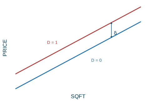
The single coefficient $\delta$ does all the work. To see what it means, write out the regression function <80><94> the conditional mean <80><94> for each value of the dummy. It splits into two cases: \[ \E(\text{PRICE}\given\text{SQFT}) = \begin{cases} (\beta_1 + \delta) + \beta_2\,\text{SQFT}, & D = 1\\[2pt] \beta_1 + \beta_2\,\text{SQFT}, & D = 0 . \end{cases} \] The two lines have the same slope $\beta_2$ but different intercepts: $\beta_1$ for houses away from campus, $\beta_1 + \delta$ for houses near it. Adding the dummy produces a parallel shift of the regression line by the amount $\delta$ (Figure 19.1).

The intercept dummy

An indicator entered on its own shifts the line up or down without tilting it. Here $\delta$ is the location premium: the price difference from being near the university, holding size fixed. It is the vertical gap between the two parallel lines.

Show the R code

xs <- seq(0.5, 9, length.out = 200)
lines_df <- rbind(
  data.frame(x = xs, y = 1.0 + 0.8 * xs, grp = "D = 0"),
  data.frame(x = xs, y = 2.5 + 0.8 * xs, grp = "D = 1")
)
ggplot(lines_df, aes(x, y, color = grp)) +
  geom_line(linewidth = 1) +
  annotate("segment", x = 7, xend = 7, y = 1.0 + 0.8 * 7, yend = 2.5 + 0.8 * 7,
           color = ucla$darkblue,
           arrow = arrow(ends = "both", length = unit(0.12, "cm"))) +
  annotate("text", x = 7.25, y = 7.05, label = "delta",
           parse = TRUE, color = ucla$darkblue, size = 4) +
  annotate("text", x = 3, y = 6.1, label = "D = 1", color = ucla$red, size = 3.6) +
  annotate("text", x = 6, y = 4.3, label = "D = 0", color = ucla$blue, size = 3.6) +
  scale_color_manual(values = c("D = 0" = ucla$blue, "D = 1" = ucla$red)) +
  scale_x_continuous(breaks = NULL) +
  scale_y_continuous(breaks = NULL) +
  labs(x = "SQFT", y = "PRICE") +
  theme(legend.position = "none")

Figure 19.1: An intercept dummy shifts the regression line in parallel by the premium $\delta$.

The reference group

Because the dummy is $0$ for one of the two groups, that group has no extra term: it is the base (or reference) group, the omitted category that everyone else is compared to. The coefficient $\delta$ is the gap relative to the base. Which group plays the role of the base is entirely your choice <80><94> pick whichever makes the comparison you want to report most convenient.

Reference group

When a single indicator $D$ is included, the category with $D = 0$ is the reference group. Every coefficient on a dummy measures a difference relative to that omitted group, holding the other regressors fixed.

The dummy-variable trap

There is one mistake to avoid. Do not include both $D$ and its opposite $(1 - D)$ alongside the intercept. Those two indicators add up to $1$ for every observation, which is exactly the constant the intercept already supplies. They are therefore perfectly collinear with the constant column, and the no-perfect-collinearity assumption (MR5) fails <80><94> OLS cannot separate their effects and the estimates are not defined.

The dummy-variable trap

With an intercept in the model, include only one indicator from a two-way split. The omitted category automatically becomes the base. Keeping both $D$ and $1 - D$ creates perfect collinearity with the constant and breaks OLS.

Apart from this caveat, a dummy is treated like any other regressor. The coefficient $\delta$ has a standard error, a $t$-statistic (so we can ask “is the premium statistically significant?”), and a confidence interval. None of the inference mechanics is new; only the reading of the coefficient <80><94> as a group difference rather than a marginal effect of a continuous variable <80><94> is special.

19.2 Slope dummies

The intercept dummy assumes the value per square foot is the same near and away from campus, and only the base level differs. But maybe location changes the slope itself <80><94> perhaps each additional square foot is worth more near the university. To allow that, interact the dummy with the continuous regressor: \[ \text{PRICE} = \beta_1 + \beta_2\,\text{SQFT} + \gamma\,(\text{SQFT}\times D) + e . \]

Now differentiate the regression function with respect to SQFT to read off the slope for each group: \[ \frac{\partial\,\E(\text{PRICE})}{\partial\,\text{SQFT}} = \begin{cases} \beta_2 + \gamma, & D = 1\\[2pt] \beta_2, & D = 0 . \end{cases} \] The coefficient $\gamma$ is the difference in slopes <80><94> the extra value of a square foot near the university. The product term $\text{SQFT}\times D$ is called a slope-indicator, or slope dummy, variable.

Intercept dummy vs. slope dummy

An intercept dummy $\delta D$ shifts the line (same slope, different height). A slope dummy $\gamma(x \times D)$ tilts it (same height at $x=0$, different slope). They answer different questions: does the group start higher? versus does the group’s variable matter more?

We need not choose. Including both an intercept dummy and a slope dummy, \[ \text{PRICE} = \beta_1 + \delta D + \beta_2\,\text{SQFT} + \gamma\,(\text{SQFT}\times D) + e , \] gives each group its own intercept and its own slope. This single regression is then exactly equivalent to running two completely separate regressions, one on each subsample <80><94> which is the idea behind the Chow test for whether two groups share the same regression.

Worked example: the university effect

The HGL utown data record $N = 1000$ home sales. We regress PRICE on the UTOWN intercept dummy, SQFT, the slope dummy SQFT$\times$UTOWN, and three more characteristics: AGE, an intercept dummy POOL for whether the house has a pool, and an intercept dummy FPLACE for a fireplace. PRICE is measured in thousands of dollars and SQFT in hundreds of square feet.

data(utown)
fit <- lm(price ~ utown + sqft + I(sqft * utown) + age + pool + fplace,
          data = utown)
round(coef(fit), 3)
#>     (Intercept)           utown            sqft I(sqft * utown)             age 
#>          24.500          27.453           7.612           1.299          -0.190 
#>            pool          fplace 
#>           4.377           1.649

The estimates line up with the slide table to three decimals (UTOWN $27.45$, SQFT $7.61$, slope $1.30$, AGE $-0.19$, POOL $4.38$, FPLACE $1.65$), and the fit is tight, $R^2 = 0.87$, with every term significant on a one-tailed test except FPLACE, which is borderline. Reading the coefficients back into dollars:

Location premium. The UTOWN intercept dummy is $27.45$, so a house near the university sells for about $27,453 more, holding size and the other features fixed.
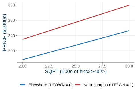
Price per 100 ft. Away from campus an extra $100$ ft adds $7.61$, or $7,612; near campus the slope dummy adds $1.30$ on top, so the value of $100$ ft rises to $7.61 + 1.30 = 8.91$, about $8,912. The slope dummy is worth an extra $1,299 per $100$ ft near the university.
Other features. Each year of age lowers price by $0.19$ ($-\$190$); a pool adds $4.38$ ($+\$4,377$); a fireplace adds $1.65$ ($+\$1,649$).

POOL and FPLACE are pure intercept dummies (level shifts), while UTOWN enters both as an intercept dummy and, through SQFT$\times$UTOWN, as a slope dummy. This is the same binary-interaction machinery introduced with interaction terms.

Figure 19.2 shows the two fitted price<80><93>size lines that result, one for houses near the university and one for houses elsewhere (holding AGE, POOL, and FPLACE at zero). The UTOWN line starts higher (the intercept premium) and rises more steeply (the slope premium).

Show the R code

b <- coef(fit)
sqft_grid <- seq(20, 30, length.out = 100)
util <- rbind(
  data.frame(sqft = sqft_grid,
             price = b[["(Intercept)"]] + b[["sqft"]] * sqft_grid,
             grp = "Elsewhere (UTOWN = 0)"),
  data.frame(sqft = sqft_grid,
             price = b[["(Intercept)"]] + b[["utown"]] +
               (b[["sqft"]] + b[["I(sqft * utown)"]]) * sqft_grid,
             grp = "Near campus (UTOWN = 1)")
)
ggplot(util, aes(sqft, price, color = grp)) +
  geom_line(linewidth = 1) +
  scale_color_manual(values = c("Elsewhere (UTOWN = 0)" = ucla$blue,
                                "Near campus (UTOWN = 1)" = ucla$red)) +
  labs(x = "SQFT (100s of ft<c2><b2>)", y = "PRICE ($1000s)", color = NULL)

Figure 19.2: Fitted price<80><93>size lines from the `utown` regression: near campus the line is both higher and steeper.

19.3 Several categories and joint tests

So far the qualitative factor had only two levels. What if it has more <80><94> say a region with four categories, Northeast, South, Midwest, and West? The rule follows directly from the dummy-variable trap: a factor with $G$ categories needs $G - 1$ dummies plus the intercept, never $G$. Including all $G$ dummies together with the constant recreates the trap, because the $G$ region indicators sum to $1$ for every observation.

For a wage equation with education and region we therefore write \[ \text{WAGE} = \beta_1 + \beta_2\,\text{EDUC} + \delta_1\,\text{SOUTH} + \delta_2\,\text{MIDWEST} + \delta_3\,\text{WEST} + e , \] omitting one region. The omitted region <80><94> here NORTHEAST <80><94> is the reference group. Each $\delta$ is that region’s wage gap relative to the Northeast, holding education fixed; for instance, a coefficient of about $-\$1.65$/hr on SOUTH would say Southern workers earn that much less than otherwise-similar Northeastern workers. The choice of base is arbitrary: changing which region is omitted changes only which comparisons the coefficients report, not the underlying fit or predictions.

How many dummies for $G$ categories

A categorical factor with $G$ levels requires exactly $G - 1$ indicator variables when the model contains an intercept. The omitted level is the reference group, and each coefficient is a difference relative to it. Keeping all $G$ dummies triggers the dummy-variable trap.

Testing a whole categorical factor

A natural question is whether the factor matters at all <80><94> is there any regional effect on wages? This is not a question about one coefficient but about all of them at once, a joint hypothesis: \[ H_0:\ \delta_1 = \delta_2 = \delta_3 = 0 . \] The right tool is an $F$-test of all the region dummies jointly, not three separate $t$-tests. (Running several $t$-tests inflates the chance of a false positive and cannot answer the joint question.) For the wage data the test gives $F = 1.58$ with $p = 0.19$, so we fail to reject $H_0$: there is no statistically significant regional difference in this sample once education is controlled for.

The $F$-test for several dummies is the same joint-restriction test developed in the chapter on $F$-tests; region dummies are simply a common place it shows up.

Dummies can interact with each other

Indicators interact with each other just as they interact with continuous variables. Suppose we want the wage gap specific to Black women. Including separate BLACK and FEMALE dummies will not capture it <80><94> those measure the gaps for being Black (averaged over sex) and for being female (averaged over race), not the combination. To let the combination differ, add the product BLACK$\times$FEMALE.

Interacting two indicators

With BLACK, FEMALE, and BLACK$\times$FEMALE in the model, each of the four cells <80><94> white male, Black male, white female, Black female <80><94> gets its own intercept, read off as a sum of coefficients. The product term is what lets the female penalty differ by race (and the race penalty differ by sex).

19.4 The linear probability model

Everything above put the indicator on the right-hand side, as a regressor. Now flip it to the left-hand side. Many outcomes we care about are themselves yes/no: a mortgage application is denied or not, a shopper buys Coke or Pepsi, a student goes to college or not. Let the dependent variable $y \in \{0, 1\}$.

What does it mean to run a regression on a binary $y$? Take the conditional expectation of a $0/1$ variable: \[ \E(y\given X) = 1\cdot\Prob(y = 1\given X) + 0\cdot\Prob(y = 0\given X) = \Prob(y = 1\given X) . \] The conditional mean of a binary variable is the conditional probability that it equals one. So when we model $\E(y\given X)$ with a regression line, we are modeling a probability. This is the linear probability model (LPM): \[ \Prob(y = 1\given X) = \beta_1 + \beta_2 x_2 + \dots + \beta_K x_K . \]

Linear probability model (LPM)

When the dependent variable is binary, OLS fits $\Prob(y = 1 \given X)$ as a linear function of the regressors. Each coefficient $\beta_k$ is the change in the probability that $y = 1$ for a one-unit increase in $x_k$, holding the others fixed. It is estimated by OLS, exactly as before.

Example: mortgage denial

Does an applicant’s race affect the chance a mortgage is denied, holding the payment-to-income (P/I) ratio fixed? Using the Boston HMDA data with $y = \text{deny}$, OLS produces \[ \widehat{\text{deny}} = -0.091 + 0.559\,(\text{P/I ratio}) + 0.177\,\text{black} . \] Reading the coefficients as changes in the denial probability:

A $0.1$ rise in the P/I ratio raises the denial probability by about $0.559 \times 0.1 \approx 0.056$, or 5.6 percentage points.
Holding the P/I ratio fixed, a Black applicant’s denial probability is 17.7 percentage points higher than a white applicant’s, and the difference is sharply significant ($t = 7.1$).

Suggestive, not proof

A large, significant black coefficient is suggestive of discrimination but is not proof of it. Credit history and many other determinants of denial are omitted from this regression, so omitted-variable bias is a live worry. The coefficient is a starting point for investigation, not a verdict.

The limits of the LPM

The linearity that makes the LPM so easy to estimate and interpret is also its weakness. There are three problems.

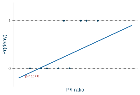
Predicted probabilities can leave $[0, 1]$. A straight line, extended far enough, will eventually predict $\hat p < 0$ or $\hat p > 1$ <80><94> nonsense for a probability. Figure 19.3 shows the fitted line dipping below $0$ at low P/I ratios.
The errors are heteroskedastic. For a binary outcome the conditional variance is $\Var(e \given X) = p(1 - p)$, which depends on $X$ through $p$. The constant-variance assumption (SR3/MR3) therefore fails automatically, and the usual standard errors are wrong. The fix is to use robust standard errors.
$R^2$ is not meaningful. Because the points all sit at $y = 0$ or $y = 1$, they can never line up on a straight line, so the usual goodness-of- fit measure does not have its normal interpretation.

Show the R code

pts <- data.frame(
  x = c(0.10, 0.20, 0.25, 0.35, 0.40, 0.45, 0.55, 0.60, 0.70),
  y = c(0,    0,    0,    0,    1,    0,    1,    1,    1)
)
line_df <- data.frame(x = c(0, 1), y = c(-0.2, 0.9))
ggplot() +
  geom_hline(yintercept = c(0, 1), linetype = "dashed", color = ucla$gray) +
  geom_line(data = line_df, aes(x, y), color = ucla$blue, linewidth = 1) +
  geom_point(data = pts, aes(x, y), color = ucla$darkblue, size = 1.6) +
  annotate("text", x = 0.12, y = -0.16, label = "p-hat < 0",
           color = ucla$red, size = 3.2) +
  scale_x_continuous(breaks = NULL, limits = c(0, 1)) +
  scale_y_continuous(breaks = c(0, 1), limits = c(-0.3, 1.3)) +
  labs(x = "P/I ratio", y = "Pr(deny)")

Figure 19.3: An LPM fit can predict probabilities outside $[0,1]$: the line dips below 0 and rises above 1.

Despite these flaws, the LPM estimates marginal effects well as long as the fitted probabilities are not near $0$ or $1$, and it is wonderfully transparent <80><94> a coefficient is just a change in probability.

The proper fix for the out-of-bounds problem is to replace the straight line with an S-shaped curve that stays inside $(0, 1)$ <80><94> the probit and logit models. Those are beyond this course (HGL ch. 16, S&W 11.2).

19.5 Recap

Indicator variables let qualitative factors enter a regression with no change to the OLS machinery <80><94> only to interpretation.

Dummies as regressors.

An intercept dummy $\delta D$ produces a parallel shift, a group premium measured against the base group ($D = 0$).
A slope dummy $\gamma(x \times D)$ gives a group its own slope; including both lets a group have its own intercept and slope.
In the utown data, being near the university adds a $27.5k premium and raises the value of $100$ ft from $7,612 to $8,912.
A factor with $G$ categories needs $G - 1$ dummies plus the intercept <80><94> keeping all $G$ is the dummy-variable trap <80><94> and the factor as a whole is tested with an $F$-test.

Binary $y$: the linear probability model.

$\Prob(y = 1 \given X) = \beta_1 + \beta_2 x_2 + \dots$, and each coefficient is a change in probability.
In the mortgage data, a Black applicant’s denial probability is $17.7$ percentage points higher, holding the P/I ratio fixed.
Its flaws: $\hat p$ can fall outside $[0, 1]$, the errors are heteroskedastic (use robust standard errors), and $R^2$ is not meaningful.

Next time: the most important dummy of all <80><94> the treatment indicator. With potential outcomes, the average treatment effect, and randomization (Project STAR), we will see exactly when a regression coefficient is truly causal in treatment effects and difference-in-differences.

--- title: "Indicator (Dummy) Variables" --- {{< include _setup.qmd >}} > **Reading.** SW sec. 5.3, 8.3, 11.1, HGL sec. 7.1--7.2, 7.4 Every regressor so far has been **quantitative** --- income, price, square footage. But many of the things that drive economic outcomes are **qualitative**: a house's *neighborhood*, a worker's *sex* or *region*, whether a person *received a treatment*. These factors are categories, not numbers, yet they clearly belong in our models. The trick is to encode a qualitative factor as a **0/1 indicator** --- a *dummy* variable --- and then let it drop straight into OLS. Nothing about the estimation machinery changes; only the *interpretation* of the coefficient does. This chapter develops three uses of indicators. First, **intercept dummies**, which shift the regression line up or down by a group "premium" measured against a *reference group*. Second, **slope dummies**, which let different groups have different slopes. Finally, we flip the idea around: when $y$ *itself* is binary, OLS becomes the **linear probability model** --- useful, transparent, and limited. This is the qualitative-data payoff of the [interaction machinery](16-interactions.qmd) and sets up the most important indicator of all, the [treatment indicator](20-treatment-effects.qmd) of the next chapter. ## Intercept dummies {#sec-intercept-dummies} Start from a **hedonic** house-price model, in which a house's price is explained by its characteristics: $$ \text{PRICE} = \beta_1 + \beta_2\,\text{SQFT} + e . $$ Does being near a university add value? "Near the university" is a yes/no trait, so we encode it as an indicator: let $D = 1$ if the house is near the university and $D = 0$ otherwise. Adding it to the model gives $$ \text{PRICE} = \beta_1 + \delta D + \beta_2\,\text{SQFT} + e . $$ The single coefficient $\delta$ does all the work. To see what it means, write out the regression function --- the conditional mean --- for each value of the dummy. It splits into two cases: $$ \E(\text{PRICE}\given\text{SQFT}) = \begin{cases} (\beta_1 + \delta) + \beta_2\,\text{SQFT}, & D = 1\\[2pt] \beta_1 + \beta_2\,\text{SQFT}, & D = 0 . \end{cases} $$ The two lines have the **same slope** $\beta_2$ but **different intercepts**: $\beta_1$ for houses away from campus, $\beta_1 + \delta$ for houses near it. Adding the dummy produces a **parallel shift** of the regression line by the amount $\delta$ (@fig-intercept-dummy). ::: {.keyidea title="The intercept dummy"} An indicator entered on its own shifts the line up or down without tilting it. Here $\delta$ is the **location premium**: the price difference from being near the university, holding size fixed. It is the vertical gap between the two parallel lines. ::: ```{r} #| label: fig-intercept-dummy #| fig-cap: "An intercept dummy shifts the regression line in parallel by the premium $\\delta$." #| fig-width: 5 #| fig-height: 3.4 xs <- seq(0.5, 9, length.out = 200) lines_df <- rbind( data.frame(x = xs, y = 1.0 + 0.8 * xs, grp = "D = 0"), data.frame(x = xs, y = 2.5 + 0.8 * xs, grp = "D = 1") ) ggplot(lines_df, aes(x, y, color = grp)) + geom_line(linewidth = 1) + annotate("segment", x = 7, xend = 7, y = 1.0 + 0.8 * 7, yend = 2.5 + 0.8 * 7, color = ucla$darkblue, arrow = arrow(ends = "both", length = unit(0.12, "cm"))) + annotate("text", x = 7.25, y = 7.05, label = "delta", parse = TRUE, color = ucla$darkblue, size = 4) + annotate("text", x = 3, y = 6.1, label = "D = 1", color = ucla$red, size = 3.6) + annotate("text", x = 6, y = 4.3, label = "D = 0", color = ucla$blue, size = 3.6) + scale_color_manual(values = c("D = 0" = ucla$blue, "D = 1" = ucla$red)) + scale_x_continuous(breaks = NULL) + scale_y_continuous(breaks = NULL) + labs(x = "SQFT", y = "PRICE") + theme(legend.position = "none") ``` ### The reference group Because the dummy is $0$ for one of the two groups, that group has no extra term: it is the **base** (or **reference**) group, the omitted category that everyone else is compared *to*. The coefficient $\delta$ is the gap *relative to the base*. Which group plays the role of the base is entirely your choice --- pick whichever makes the comparison you want to report most convenient. ::: {.definition title="Reference group"} When a single indicator $D$ is included, the category with $D = 0$ is the **reference group**. Every coefficient on a dummy measures a difference *relative to that omitted group*, holding the other regressors fixed. ::: ### The dummy-variable trap There is one mistake to avoid. Do not include *both* $D$ and its opposite $(1 - D)$ alongside the intercept. Those two indicators add up to $1$ for every observation, which is exactly the constant the intercept already supplies. They are therefore **perfectly collinear** with the constant column, and the no-perfect-collinearity assumption (MR5) fails --- OLS cannot separate their effects and the estimates are not defined. ::: {.warningbox title="The dummy-variable trap"} With an intercept in the model, include only **one** indicator from a two-way split. The omitted category automatically becomes the base. Keeping both $D$ and $1 - D$ creates **perfect collinearity** with the constant and breaks OLS. ::: Apart from this caveat, a dummy is treated like any other regressor. The coefficient $\delta$ has a standard error, a $t$-statistic (so we can ask "is the premium statistically significant?"), and a confidence interval. None of the inference mechanics is new; only the *reading* of the coefficient --- as a **group difference** rather than a marginal effect of a continuous variable --- is special. ## Slope dummies {#sec-slope-dummies} The intercept dummy assumes the *value per square foot* is the same near and away from campus, and only the base level differs. But maybe location changes the slope itself --- perhaps each additional square foot is worth more near the university. To allow that, **interact** the dummy with the continuous regressor: $$ \text{PRICE} = \beta_1 + \beta_2\,\text{SQFT} + \gamma\,(\text{SQFT}\times D) + e . $$ Now differentiate the regression function with respect to SQFT to read off the slope for each group: $$ \frac{\partial\,\E(\text{PRICE})}{\partial\,\text{SQFT}} = \begin{cases} \beta_2 + \gamma, & D = 1\\[2pt] \beta_2, & D = 0 . \end{cases} $$ The coefficient $\gamma$ is the **difference in slopes** --- the extra value of a square foot near the university. The product term $\text{SQFT}\times D$ is called a **slope-indicator**, or *slope dummy*, variable. ::: {.keyidea title="Intercept dummy vs. slope dummy"} An **intercept dummy** $\delta D$ shifts the line (same slope, different height). A **slope dummy** $\gamma(x \times D)$ tilts it (same height at $x=0$, different slope). They answer different questions: *does the group start higher?* versus *does the group's variable matter more?* ::: We need not choose. Including *both* an intercept dummy and a slope dummy, $$ \text{PRICE} = \beta_1 + \delta D + \beta_2\,\text{SQFT} + \gamma\,(\text{SQFT}\times D) + e , $$ gives each group its **own intercept and its own slope**. This single regression is then exactly equivalent to running two completely separate regressions, one on each subsample --- which is the idea behind the **Chow test** for whether two groups share the same regression. ### Worked example: the university effect The HGL `utown` data record $N = 1000$ home sales. We regress PRICE on the UTOWN intercept dummy, SQFT, the slope dummy SQFT$\times$UTOWN, and three more characteristics: AGE, an intercept dummy POOL for whether the house has a pool, and an intercept dummy FPLACE for a fireplace. PRICE is measured in thousands of dollars and SQFT in hundreds of square feet. ```{r} #| label: utown-fit #| code-fold: false data(utown) fit <- lm(price ~ utown + sqft + I(sqft * utown) + age + pool + fplace, data = utown) round(coef(fit), 3) ``` The estimates line up with the slide table to three decimals (UTOWN $27.45$, SQFT $7.61$, slope $1.30$, AGE $-0.19$, POOL $4.38$, FPLACE $1.65$), and the fit is tight, $R^2 = 0.87$, with every term significant on a one-tailed test except FPLACE, which is borderline. Reading the coefficients back into dollars: - **Location premium.** The UTOWN intercept dummy is $27.45$, so a house near the university sells for about **\$27,453** more, holding size and the other features fixed. - **Price per 100 ft^2.** Away from campus an extra $100$ ft^2 adds $7.61$, or **\$7,612**; near campus the slope dummy adds $1.30$ on top, so the value of $100$ ft^2 rises to $7.61 + 1.30 = 8.91$, about **\$8,912**. The slope dummy is worth an extra **\$1,299** per $100$ ft^2 near the university. - **Other features.** Each year of age lowers price by $0.19$ ($-\$190$); a pool adds $4.38$ ($+\$4,377$); a fireplace adds $1.65$ ($+\$1,649$). ::: {.callout-note appearance="simple"} POOL and FPLACE are pure **intercept** dummies (level shifts), while UTOWN enters **both** as an intercept dummy and, through SQFT$\times$UTOWN, as a slope dummy. This is the same binary-interaction machinery introduced with [interaction terms](16-interactions.qmd). ::: @fig-utown shows the two fitted price--size lines that result, one for houses near the university and one for houses elsewhere (holding AGE, POOL, and FPLACE at zero). The UTOWN line starts higher (the intercept premium) *and* rises more steeply (the slope premium). ```{r} #| label: fig-utown #| fig-cap: "Fitted price--size lines from the `utown` regression: near campus the line is both higher and steeper." #| fig-width: 5 #| fig-height: 3.4 b <- coef(fit) sqft_grid <- seq(20, 30, length.out = 100) util <- rbind( data.frame(sqft = sqft_grid, price = b[["(Intercept)"]] + b[["sqft"]] * sqft_grid, grp = "Elsewhere (UTOWN = 0)"), data.frame(sqft = sqft_grid, price = b[["(Intercept)"]] + b[["utown"]] + (b[["sqft"]] + b[["I(sqft * utown)"]]) * sqft_grid, grp = "Near campus (UTOWN = 1)") ) ggplot(util, aes(sqft, price, color = grp)) + geom_line(linewidth = 1) + scale_color_manual(values = c("Elsewhere (UTOWN = 0)" = ucla$blue, "Near campus (UTOWN = 1)" = ucla$red)) + labs(x = "SQFT (100s of ft^2)", y = "PRICE ($1000s)", color = NULL) ``` ## Several categories and joint tests {#sec-categories} So far the qualitative factor had only two levels. What if it has more --- say a region with four categories, Northeast, South, Midwest, and West? The rule follows directly from the dummy-variable trap: a factor with $G$ categories needs **$G - 1$ dummies** plus the intercept, never $G$. Including all $G$ dummies together with the constant recreates the trap, because the $G$ region indicators sum to $1$ for every observation. For a wage equation with education and region we therefore write $$ \text{WAGE} = \beta_1 + \beta_2\,\text{EDUC} + \delta_1\,\text{SOUTH} + \delta_2\,\text{MIDWEST} + \delta_3\,\text{WEST} + e , $$ omitting one region. The omitted region --- here **NORTHEAST** --- is the reference group. Each $\delta$ is that region's wage gap *relative to the Northeast*, holding education fixed; for instance, a coefficient of about $-\$1.65$/hr on SOUTH would say Southern workers earn that much less than otherwise-similar Northeastern workers. The choice of base is arbitrary: changing which region is omitted changes only which *comparisons* the coefficients report, not the underlying fit or predictions. ::: {.property title="How many dummies for $G$ categories"} A categorical factor with $G$ levels requires exactly **$G - 1$** indicator variables when the model contains an intercept. The omitted level is the reference group, and each coefficient is a difference relative to it. Keeping all $G$ dummies triggers the dummy-variable trap. ::: ### Testing a whole categorical factor A natural question is whether the factor matters *at all* --- is there **any** regional effect on wages? This is not a question about one coefficient but about *all of them at once*, a joint hypothesis: $$ H_0:\ \delta_1 = \delta_2 = \delta_3 = 0 . $$ The right tool is an **$F$-test** of all the region dummies jointly, not three separate $t$-tests. (Running several $t$-tests inflates the chance of a false positive and cannot answer the joint question.) For the wage data the test gives $F = 1.58$ with $p = 0.19$, so we **fail to reject** $H_0$: there is no statistically significant regional difference in this sample once education is controlled for. ::: {.callout-note appearance="simple"} The $F$-test for several dummies is the same joint-restriction test developed in the chapter on [$F$-tests](17-ftests.qmd); region dummies are simply a common place it shows up. ::: ### Dummies can interact with each other Indicators interact with each other just as they interact with continuous variables. Suppose we want the wage gap specific to **Black women**. Including separate BLACK and FEMALE dummies will not capture it --- those measure the gaps for being Black (averaged over sex) and for being female (averaged over race), not the combination. To let the combination differ, add the product BLACK$\times$FEMALE. ::: {.keyidea title="Interacting two indicators"} With BLACK, FEMALE, and BLACK$\times$FEMALE in the model, each of the four cells --- white male, Black male, white female, Black female --- gets its **own intercept**, read off as a sum of coefficients. The product term is what lets the female penalty differ by race (and the race penalty differ by sex). ::: ## The linear probability model {#sec-lpm} Everything above put the indicator on the **right-hand side**, as a regressor. Now flip it to the **left-hand side**. Many outcomes we care about are themselves yes/no: a mortgage application is *denied* or not, a shopper buys Coke or Pepsi, a student goes to college or not. Let the dependent variable $y \in \{0, 1\}$. What does it mean to run a regression on a binary $y$? Take the conditional expectation of a $0/1$ variable: $$ \E(y\given X) = 1\cdot\Prob(y = 1\given X) + 0\cdot\Prob(y = 0\given X) = \Prob(y = 1\given X) . $$ The conditional mean of a binary variable *is* the conditional probability that it equals one. So when we model $\E(y\given X)$ with a regression line, we are modeling a **probability**. This is the **linear probability model** (LPM): $$ \Prob(y = 1\given X) = \beta_1 + \beta_2 x_2 + \dots + \beta_K x_K . $$ ::: {.definition title="Linear probability model (LPM)"} When the dependent variable is binary, OLS fits $\Prob(y = 1 \given X)$ as a linear function of the regressors. Each coefficient $\beta_k$ is the **change in the probability that $y = 1$** for a one-unit increase in $x_k$, holding the others fixed. It is estimated by OLS, exactly as before. ::: ### Example: mortgage denial Does an applicant's race affect the chance a mortgage is denied, holding the payment-to-income (P/I) ratio fixed? Using the Boston HMDA data with $y = \text{deny}$, OLS produces $$ \widehat{\text{deny}} = -0.091 + 0.559\,(\text{P/I ratio}) + 0.177\,\text{black} . $$ Reading the coefficients as changes in the denial probability: - A $0.1$ rise in the P/I ratio raises the denial probability by about $0.559 \times 0.1 \approx 0.056$, or **5.6 percentage points**. - Holding the P/I ratio fixed, a Black applicant's denial probability is **17.7 percentage points higher** than a white applicant's, and the difference is sharply significant ($t = 7.1$). ::: {.warningbox title="Suggestive, not proof"} A large, significant `black` coefficient is *suggestive* of discrimination but is **not** proof of it. Credit history and many other determinants of denial are omitted from this regression, so [omitted-variable bias](18-model-specification.qmd) is a live worry. The coefficient is a starting point for investigation, not a verdict. ::: ### The limits of the LPM The linearity that makes the LPM so easy to estimate and interpret is also its weakness. There are three problems. 1. **Predicted probabilities can leave $[0, 1]$.** A straight line, extended far enough, will eventually predict $\hat p < 0$ or $\hat p > 1$ --- nonsense for a probability. @fig-lpm shows the fitted line dipping below $0$ at low P/I ratios. 2. **The errors are heteroskedastic.** For a binary outcome the conditional variance is $\Var(e \given X) = p(1 - p)$, which depends on $X$ through $p$. The constant-variance assumption (SR3/MR3) therefore fails automatically, and the usual standard errors are wrong. The fix is to use **robust standard errors**. 3. **$R^2$ is not meaningful.** Because the points all sit at $y = 0$ or $y = 1$, they can never line up on a straight line, so the usual goodness-of- fit measure does not have its normal interpretation. ```{r} #| label: fig-lpm #| fig-cap: "An LPM fit can predict probabilities outside $[0,1]$: the line dips below 0 and rises above 1." #| fig-width: 5 #| fig-height: 3.4 pts <- data.frame( x = c(0.10, 0.20, 0.25, 0.35, 0.40, 0.45, 0.55, 0.60, 0.70), y = c(0, 0, 0, 0, 1, 0, 1, 1, 1) ) line_df <- data.frame(x = c(0, 1), y = c(-0.2, 0.9)) ggplot() + geom_hline(yintercept = c(0, 1), linetype = "dashed", color = ucla$gray) + geom_line(data = line_df, aes(x, y), color = ucla$blue, linewidth = 1) + geom_point(data = pts, aes(x, y), color = ucla$darkblue, size = 1.6) + annotate("text", x = 0.12, y = -0.16, label = "p-hat < 0", color = ucla$red, size = 3.2) + scale_x_continuous(breaks = NULL, limits = c(0, 1)) + scale_y_continuous(breaks = c(0, 1), limits = c(-0.3, 1.3)) + labs(x = "P/I ratio", y = "Pr(deny)") ``` Despite these flaws, the LPM estimates **marginal effects** well as long as the fitted probabilities are not near $0$ or $1$, and it is wonderfully transparent --- a coefficient is just a change in probability. ::: {.callout-note appearance="simple"} The proper fix for the out-of-bounds problem is to replace the straight line with an S-shaped curve that stays inside $(0, 1)$ --- the **probit** and **logit** models. Those are beyond this course (HGL ch. 16, S&W sec. 11.2). ::: ## Recap {#sec-recap} Indicator variables let qualitative factors enter a regression with no change to the OLS machinery --- only to interpretation. **Dummies as regressors.** - An **intercept dummy** $\delta D$ produces a parallel shift, a group premium measured against the base group ($D = 0$). - A **slope dummy** $\gamma(x \times D)$ gives a group its own slope; including both lets a group have its own intercept *and* slope. - In the `utown` data, being near the university adds a **\$27.5k** premium and raises the value of $100$ ft^2 from **\$7,612 to \$8,912**. - A factor with $G$ categories needs $G - 1$ dummies plus the intercept --- keeping all $G$ is the dummy-variable trap --- and the factor as a whole is tested with an [$F$-test](17-ftests.qmd). **Binary $y$: the linear probability model.** - $\Prob(y = 1 \given X) = \beta_1 + \beta_2 x_2 + \dots$, and each coefficient is a change in probability. - In the mortgage data, a Black applicant's denial probability is $17.7$ percentage points higher, holding the P/I ratio fixed. - Its flaws: $\hat p$ can fall outside $[0, 1]$, the errors are heteroskedastic (use robust standard errors), and $R^2$ is not meaningful. **Next time:** the most important dummy of all --- the **treatment indicator**. With potential outcomes, the average treatment effect, and **randomization** (Project STAR), we will see exactly when a regression coefficient is truly *causal* in [treatment effects and difference-in-differences](20-treatment-effects.qmd).