\( \newcommand{\E}{\mathbb{E}} \newcommand{\Var}{\operatorname{Var}} \newcommand{\Cov}{\operatorname{Cov}} \newcommand{\Prob}{\mathbb{P}} \newcommand{\R}{\mathbb{R}} \newcommand{\given}{\,\vert\,} \newcommand{\indic}[1]{\mathbf{1}\!\left\{#1\right\}} \newcommand{\pmf}{\text{p.m.f.}} \newcommand{\pdf}{\text{p.d.f.}} \newcommand{\cdf}{\text{c.d.f.}} \)

17  F-Tests & Joint Hypothesis Testing

Reading. Hill, Griffiths & Lim (5th ed.), sec. 6.1–6.2; Stock & Watson (4th ed.), sec. 7.2.

The \(t\)-test we have used so far handles a single restriction — one “equals” sign, even one that spans several coefficients. But many of the questions we actually want to ask are joint: they impose two or more restrictions at once. Does advertising matter at all — is \(\beta_3 = 0\) and \(\beta_4 = 0\) in Big Andy’s quadratic sales model? Does a whole group of variables (socioeconomic controls, prices of substitutes) belong? Does the model explain anything — are all the slopes zero? Each of these has several equals signs, and a \(t\)-test cannot do them. Testing one restriction at a time is unreliable. The tool for the job is the \(F\)-test.

This chapter builds the \(F\)-test from the idea of comparing two nested models — one with the restrictions imposed and one without. We use it to test overall model significance, work out exactly when the \(t\)- and \(F\)-tests agree, and finally turn it loose on economic restrictions like constant returns to scale. It builds directly on the multiple-regression machinery and single-coefficient tests of multiple-regression hypothesis testing.

17.1 Why a new test?

A joint hypothesis imposes \(J \ge 2\) restrictions simultaneously. A typical example in Big Andy’s model is \[ H_0:\ \beta_3 = 0 \ \text{ and } \ \beta_4 = 0 \qquad\text{vs.}\qquad H_1:\ \beta_3 \neq 0 \ \text{ or } \ \beta_4 \neq 0 . \] Notice the asymmetry: the null requires both coefficients to be zero, while the alternative needs only one of them to be nonzero.

The natural temptation is to just run two separate \(t\)-tests, one for each coefficient, and combine the verdicts. This is a trap.

Why two t-tests are not a joint test

• Error rates compound. Two separate \(5\%\) tests do not deliver a \(5\%\) joint test. The chance of some false rejection across the two is larger than \(5\%\), so the combined procedure has the wrong size.
• It misreads correlated regressors. When two regressors are collinear, each individual \(t\) can come out insignificant while the pair is jointly decisive. A one-at-a-time procedure would wrongly drop both, throwing away variables that genuinely belong.

We need a test that weighs all the restrictions together, in a single statistic with a single \(p\)-value. That is the \(F\)-test.

17.2 The F-statistic: restricted vs. unrestricted

The \(F\)-test compares the fit of two nested models: an unrestricted (full) model, and a restricted model obtained by imposing \(H_0\).

Two models, with and without the restrictions

Take Big Andy’s quadratic sales model. The unrestricted model is the full specification, \[ \text{SALES} = \beta_1 + \beta_2\text{PRICE} + \beta_3\text{ADVERT} + \beta_4\text{ADVERT}^2 + e , \] with sum of squared errors \(\mathrm{SSE}_U\). The restricted model imposes \(H_0:\beta_3 = \beta_4 = 0\), dropping both advertising terms, \[ \text{SALES} = \beta_1 + \beta_2\text{PRICE} + e , \] with sum of squared errors \(\mathrm{SSE}_R\).

Dropping variables can only worsen the fit — OLS on the full model is free to set those coefficients to zero if that is best, so allowing them to be nonzero can never increase the squared-error total. Hence \[ \mathrm{SSE}_R \ge \mathrm{SSE}_U \quad\text{always.} \] The whole question is whether the increase in SSE from imposing \(H_0\) is large or small. A large increase means the restrictions hurt the fit a lot — the dropped variables mattered — so we reject \(H_0\). A small increase means the restrictions were nearly harmless, and we do not reject.

The \(F\)-statistic turns “how big is the increase?” into a number with a known distribution.

The F-statistic

\[ F = \frac{(\mathrm{SSE}_R - \mathrm{SSE}_U)/J}{\mathrm{SSE}_U/(N-K)} \;\sim\; F_{(J,\,N-K)} \quad\text{under } H_0 , \] where \(J\) is the number of restrictions (the numerator degrees of freedom) and \(N-K\) is the unrestricted model’s degrees of freedom (the denominator degrees of freedom).

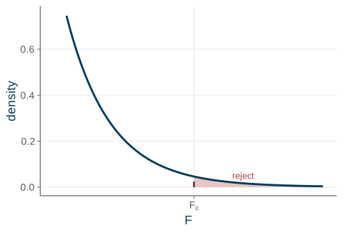
Reading the pieces: the numerator is the extra error caused by imposing \(H_0\), expressed per restriction. The denominator is the model’s own noise, \(\hat\sigma^2 = \mathrm{SSE}_U/(N-K)\). So \(F\) measures the cost of the restrictions relative to the model’s underlying variability. A large \(F\) means the restrictions cost a lot relative to noise, and we reject \(H_0\) when \(F \ge F_c\), the critical value. Because only large values count against \(H_0\), the \(F\)-test is always a right-tailed test (Figure 17.1).

Code

xs   <- seq(0.001, 6, length.out = 400)
df1  <- 2; df2 <- 71
Fc   <- qf(0.95, df1, df2)
dat  <- data.frame(x = xs, y = df(xs, df1, df2))
sh   <- subset(dat, x >= Fc)
ggplot(dat, aes(x, y)) +
  geom_area(data = sh, aes(x, y), fill = ucla$red, alpha = 0.30) +
  geom_line(color = ucla$darkblue, linewidth = 1) +
  geom_segment(aes(x = Fc, xend = Fc, y = 0, yend = df(Fc, df1, df2)),
               linetype = "dashed", color = ucla$gray) +
  annotate("text", x = Fc + 1.1, y = 0.05, label = "reject",
           color = ucla$red, size = 3.4) +
  scale_x_continuous(breaks = Fc, labels = expression(F[c])) +
  scale_y_continuous(limits = c(0, 0.75)) +
  labs(x = "F", y = "density")

Figure 17.1: The F-distribution. We reject \(H_0\) for large \(F\), in the right tail beyond the critical value \(F_c\).

Big Andy’s: does advertising matter?

Put the test to work. We test \(H_0:\beta_3 = 0,\ \beta_4 = 0\) — advertising, both its linear and quadratic terms, is irrelevant — against “at least one nonzero.” Here \(J = 2\) restrictions, \(N = 75\) observations, and \(K = 4\) coefficients in the full model. The two sums of squared errors are \[ \mathrm{SSE}_U = 1532.08, \qquad \mathrm{SSE}_R = 1896.39 , \] so the statistic is \[ F = \frac{(1896.39 - 1532.08)/2}{1532.08/(75-4)} = 8.44 . \] The \(5\%\) critical value is \(F_{(0.95,\,2,\,71)} = 3.13\), and the \(p\)-value is \(0.0005\). Since \(8.44 > 3.13\) we reject \(H_0\): advertising does affect sales. Crucially, we could not have learned this cleanly from the two separate \(t\)’s, because ADVERT and ADVERT\(^2\) are collinear — exactly the situation the joint test is built for.

In R, the entire calculation is one anova() call comparing the restricted and unrestricted fits.

data(andy)
unrestricted <- lm(sales ~ price + advert + I(advert^2), data = andy)
restricted   <- lm(sales ~ price, data = andy)
anova(restricted, unrestricted)
#> Analysis of Variance Table
#> 
#> Model 1: sales ~ price
#> Model 2: sales ~ price + advert + I(advert^2)
#>   Res.Df    RSS Df Sum of Sq      F    Pr(>F)    
#> 1     73 1896.4                                  
#> 2     71 1532.1  2    364.31 8.4414 0.0005142 ***
#> ---
#> Signif. codes:  0 '***' 0.001 '**' 0.01 '*' 0.05 '.' 0.1 ' ' 1

The F column reports \(8.44\) and Pr(>F) reports the \(p\)-value of \(0.0005\) — the same numbers as the hand calculation.

An equivalent \(R^2\) form. Stock & Watson write the same statistic in terms of fit rather than SSE: \[ F = \frac{(R^2_U - R^2_R)/J}{(1-R^2_U)/(N-K)} . \] This gives the identical number — it just computes the cost of the restrictions from the \(R^2\)’s of the two models instead of their sums of squared errors.

17.3 Overall significance and the t–F link

The single most-reported \(F\)-test asks whether the regressors jointly explain anything at all. The null sets every slope to zero, \[ H_0:\ \beta_2 = \beta_3 = \dots = \beta_K = 0 \qquad\text{(the model is worthless)} . \] Under this null the restricted model keeps only the intercept, \(y_i = \beta_1 + e_i\), which OLS fits with \(\bar y\). The restricted sum of squared errors is then exactly the total sum of squares, \(\mathrm{SSE}_R = \mathrm{SST}\). With \(J = K-1\) restrictions, the statistic specializes to \[ F = \frac{(\mathrm{SST} - \mathrm{SSE})/(K-1)}{\mathrm{SSE}/(N-K)} \;\sim\; F_{(K-1,\,N-K)} . \]

Big Andy's overall F

With \(\mathrm{SST} = 3115.48\), \(\mathrm{SSE} = 1532.08\), and \(K = 4\), \[ F = \frac{(3115.48 - 1532.08)/3}{1532.08/71} = 24.46 \;\gg\; F_c = 2.73 . \] We reject decisively — at least one of PRICE, ADVERT, ADVERT\(^2\) matters. This is the overall significance \(F\) that statistical software prints on every regression output.

It is exactly the F-statistic line at the bottom of summary():

summary(unrestricted)
#> 
#> Call:
#> lm(formula = sales ~ price + advert + I(advert^2), data = andy)
#> 
#> Residuals:
#>      Min       1Q   Median       3Q      Max 
#> -12.2553  -3.1430  -0.0117   2.8513  11.8050 
#> 
#> Coefficients:
#>             Estimate Std. Error t value Pr(>|t|)    
#> (Intercept) 109.7190     6.7990  16.137  < 2e-16 ***
#> price        -7.6400     1.0459  -7.304 3.24e-10 ***
#> advert       12.1512     3.5562   3.417  0.00105 ** 
#> I(advert^2)  -2.7680     0.9406  -2.943  0.00439 ** 
#> ---
#> Signif. codes:  0 '***' 0.001 '**' 0.01 '*' 0.05 '.' 0.1 ' ' 1
#> 
#> Residual standard error: 4.645 on 71 degrees of freedom
#> Multiple R-squared:  0.5082, Adjusted R-squared:  0.4875 
#> F-statistic: 24.46 on 3 and 71 DF,  p-value: 5.6e-11

The reported F-statistic: 24.46 on 3 and 71 DF is the overall-significance test, and its tiny \(p\)-value confirms the model explains real variation in sales.

When are \(t\) and \(F\) the same?

For a single restriction the two tests are not rivals — they are the same test in two costumes.

For a single restriction (J = 1), t and F agree

A two-tailed \(t\)-test and the \(F\)-test reach the identical conclusion, because \[ F = t^2 \qquad\text{and}\qquad F_c = t_c^2 . \] Same \(p\)-value, same verdict.

For Big Andy’s, testing \(H_0:\beta_2 = 0\) (PRICE has no effect) gives a \(t\)-statistic of \(t = -7.30\). Squaring it, \(t^2 = 53.4\), which is exactly the \(F\)-statistic for that single restriction.

But there are two situations where only one of the tools works, and it pays to know which:

• One-tailed tests (\(H_1:\beta > c\)): use \(t\). Because \(F = t^2\) squares away the sign of the deviation, the \(F\)-test cannot do a one-sided alternative.
• Joint tests (\(J \ge 2\)): use \(F\). There is no single \(t\)-statistic that captures several restrictions at once.

The working rule, then: test single restrictions with \(t\), joint restrictions with \(F\).

17.4 Testing economic restrictions

The real power of the \(F\)-test is that the restrictions can be any linear equalities that economic theory hands us — not just “this coefficient is zero.” Any restriction we can write as a linear equation in the \(\beta\)’s defines a restricted model, and the same \(F\)-statistic applies.

Cobb--Douglas and constant returns to scale

A Cobb–Douglas production function \(Q = A\,L^{\beta_2} K^{\beta_3}\) becomes, in logs, \[ \ln Q = \beta_1 + \beta_2 \ln L + \beta_3 \ln K + e . \] Constant returns to scale — doubling all inputs doubles output — is exactly the linear restriction \[ H_0:\ \beta_2 + \beta_3 = 1 . \] Impose it (a restricted model with one fewer free parameter), obtain \(\mathrm{SSE}_R\), and form the \(F\) with \(J = 1\). If the data reject in favor of \(\beta_2 + \beta_3 > 1\), the technology has increasing returns to scale.

Two more examples show how naturally theory translates into restrictions.

No money illusion (HGL beer demand)

A log-log beer-demand model is \[ \ln Q = \beta_1 + \beta_2\ln P_B + \beta_3\ln P_L + \beta_4\ln P_R + \beta_5\ln I + e , \] with the prices of beer, liquor, and remaining goods, plus income. Scaling all prices and income by the same factor should leave quantity demanded unchanged — there is no money illusion — which is the restriction \[ H_0:\ \beta_2 + \beta_3 + \beta_4 + \beta_5 = 0 . \]

Is $1{,}900 the optimal ad spend?

In Big Andy’s quadratic model, the advertising optimum satisfies \(\beta_3 + 2\beta_4\,\text{ADVERT} = 1\). Evaluated at \(\text{ADVERT} = 1.9\) (i.e. $1{,}900), this is the single restriction \[ H_0:\ \beta_3 + 3.8\,\beta_4 = 1 . \] The test gives \(F = 0.94 < 3.98\), so we fail to reject: $1{,}900 is compatible with the data.

In practice there are two equivalent ways to get \(\mathrm{SSE}_R\). You can rewrite the model to embed the restriction and re-estimate it, or you can hand the restriction directly to software, which computes the \(F\) (a Wald test) and its \(p\)-value for you. To embed the optimal-ad restriction by hand, solve it for \(\beta_3 = 1 - 3.8\,\beta_4\) and substitute, which moves the \(\text{ADVERT}\) term to the left and leaves one fewer coefficient to estimate:

# H0: beta3 + 3.8*beta4 = 1  =>  substitute beta3 = 1 - 3.8*beta4.
# Moving the ADVERT term to the left changes the response, so we compute the
# F-statistic directly from the two sums of squared errors.
restricted_ad <- lm(I(sales - advert) ~ price + I(advert^2 - 3.8 * advert),
                    data = andy)
sse_R <- sum(resid(restricted_ad)^2)   # restricted: 1 fewer free coefficient
sse_U <- sum(resid(unrestricted)^2)
J <- 1; N <- nobs(unrestricted); K <- length(coef(unrestricted))
F_stat <- ((sse_R - sse_U) / J) / (sse_U / (N - K))
c(F = F_stat, p_value = pf(F_stat, J, N - K, lower.tail = FALSE))
#>         F   p_value 
#> 0.9361953 0.3365427

The \(F\)-statistic of \(0.94\) (with \(p = 0.34\)) confirms the hand result: the data have no quarrel with $1{,}900 being optimal.

Bundling several conjectures

Nothing stops a single \(H_0\) from bundling different economic claims together. Suppose Andy plans staffing on two assumptions at once: that $1{,}900 is the optimal ad spend, and that sales at PRICE \(= 6\), ADVERT \(= 1.9\) average $80{,}000. Written out, the joint null is \[ H_0:\ \beta_3 + 3.8\,\beta_4 = 1 \quad\text{and}\quad \beta_1 + 6\beta_2 + 1.9\beta_3 + 3.61\beta_4 = 80 . \] With two restrictions (\(J = 2\)) this must be an \(F\)-test — no \(t\) can do it. Here \(F = 5.74\) with \(p = 0.005\), so we reject: the two plans are jointly incompatible with the data, even though each one alone might survive on its own.

This is the everyday use of \(F\)-tests in research — bundling a model’s theoretical restrictions together and asking whether the data can live with all of them at once. A set of assumptions that each looks fine individually can still be collectively untenable.

17.5 Recap

The \(F\)-test evaluates a joint null of \(J \ge 2\) restrictions in a single statistic — something a collection of \(t\)-tests cannot do reliably. It compares a restricted and an unrestricted model through \[ F = \frac{(\mathrm{SSE}_R - \mathrm{SSE}_U)/J}{\mathrm{SSE}_U/(N-K)} \;\sim\; F_{(J,\,N-K)} , \] rejecting when the restrictions cause a large jump in SSE. For Big Andy’s advertising terms, \(F = 8.44\) rejects.

The four faces of the \(F\)-test.

Use of the \(F\)-test	Null	Big Andy’s result
Subset of slopes	\(\beta_3 = \beta_4 = 0\)	\(F = 8.44\), reject
Overall significance	all slopes \(= 0\) (restricted model is \(\bar y\))	\(F = 24.46\), reject
Economic restriction	\(\beta_3 + 3.8\beta_4 = 1\)	\(F = 0.94\), fail to reject
Bundled restrictions	optimal ad and mean sales	\(F = 5.74\), reject

On the relationship with the \(t\)-test: for a single restriction (\(J = 1\)) the two agree exactly, since \(F = t^2\) and \(F_c = t_c^2\) (PRICE: \(t = -7.30\), \(t^2 = 53.4 = F\)). But one-tailed alternatives need \(t\) (the squaring in \(F\) discards the sign), and joint nulls need \(F\) (there is no single \(t\)). Finally, the restrictions need not be “\(=0\)”: constant returns to scale (\(\beta_2 + \beta_3 = 1\)), no money illusion (\(\sum \beta = 0\)), and an optimal ad spend (\(\beta_3 + 3.8\beta_4 = 1\)) are all just linear equalities the \(F\)-test handles in stride.

Next time: the \(F\)-test assumed we already had the right model. But choosing that model is the hard part — model specification weighs omitted-variable bias against irrelevant variables, and introduces adjusted \(R^2\), AIC/BIC, the RESET test, and residual diagnostics for deciding which variables belong.