8 Estimating Error Variance & Prediction

Reading. SW sec. 4.3, HGL sec. 2.7, 4.1

In the previous chapter we showed that OLS is unbiased and, under the Gauss–Markov assumptions, BLUE — the best linear unbiased estimator. We even wrote down its sampling variance, \[ \Var(b_2 \given x) = \frac{\sigma^2}{\sum (x_i - \bar x)^2}. \] But every variance and standard error we wrote still hides one unknown: $\sigma^2$, the error variance. Until we can estimate it, those formulas are unusable. This chapter finishes the estimation toolkit. We estimate $\sigma^2$ from the residuals, use it to compute the standard errors of $b_1$ and $b_2$ at last, and then turn the fitted line to a second purpose — making a point prediction of $y$ at a new value of $x$. After this chapter we have estimates and their standard errors: the two ingredients every confidence interval and hypothesis test will need.

8.1 Estimating the error variance

The slope, the intercept, and the error variance are the three unknowns of the simple regression model, and so far we have estimated only the first two. The last one, $\sigma^2$, is what makes precision quantifiable.

Under assumption SR2, the errors have conditional mean zero, $\E(e_i \given x) = 0$. The error variance is therefore the average squared error, \[ \sigma^2 = \Var(e_i \given x) = \E(e_i^2 \given x). \] A variance is an average of squared deviations from the mean, and here the mean is zero, so the natural estimator is just the average squared error, \[ \hat\sigma^2 = \frac{\sum e_i^2}{N}. \]

One fatal problem

The errors $e_i = y_i - \beta_1 - \beta_2 x_i$ are unobservable — computing them requires the unknown $\beta_1$ and $\beta_2$. We can never form $\sum e_i^2$ directly.

The fix is the same move we have made all along: replace the unobservable error with its observable stand-in, the residual.

From errors to residuals, with a correction

Swap each error $e_i$ for its residual $\hat e_i = y_i - b_1 - b_2 x_i$, which we can compute because $b_1$ and $b_2$ are in hand. The obvious candidate is \[ \frac{\sum \hat e_i^2}{N}, \] but this turns out to be a biased estimator of $\sigma^2$. The reason is subtle but important: OLS chose $b_1$ and $b_2$ precisely to make $\sum \hat e_i^2$ as small as possible. The residuals are therefore a touch too small on average — fitting the line to the data uses up some of the variation that the errors would otherwise show. The remedy is a degrees-of-freedom correction.

Estimator of the error variance

The unbiased estimator of $\sigma^2$ divides the sum of squared residuals by $N-2$ rather than $N$: \[ \hat\sigma^2 = \frac{\sum_{i=1}^N \hat e_i^2}{N-2} = \frac{\mathrm{SSE}}{N-2}, \qquad\text{and then}\qquad \E(\hat\sigma^2 \given x) = \sigma^2 . \] Here $\mathrm{SSE} = \sum \hat e_i^2$ is the sum of squared errors (residuals).

Why subtract exactly $2$? Because we used the data to estimate $2$ parameters, $\beta_1$ and $\beta_2$, before forming the residuals. Each estimated parameter costs one degree of freedom. The quantity $N-2$ is the degrees of freedom of the regression. The same logic explains why the ordinary sample variance of a single variable divides by $N-1$: there you estimate one parameter, the mean, before squaring deviations.

The standard error of the regression

The estimator $\hat\sigma^2$ lives in the squared units of $y$, which makes it hard to interpret directly. Taking its square root returns us to the units of $y$ and gives a quantity with its own name.

Standard error of the regression (SER)

\[ \hat\sigma = \sqrt{\hat\sigma^2} \] is the standard error of the regression — the typical vertical distance of a data point from the fitted line.

How to read the SER

$\hat\sigma$ measures the typical vertical distance of a data point from the fitted line — the size of a typical residual, in the units of the dependent variable. A small SER means the points hug the line; a large SER means a loose scatter that the regression explains only partially.

Naming. Software labels this quantity in many ways: “S.E. of regression” (EViews), “Residual standard error” (R), “Root MSE” (Stata). They are all the same number, $\hat\sigma$.

Worked example: the food data

Return to the food-expenditure data (HGL Example 2.5), where the fitted line is $\hat y = 83.42 + 10.21\,x$ with $x$ measured in hundreds of dollars of weekly income. To estimate $\sigma^2$ we sum the $40$ squared residuals, \[ \mathrm{SSE} = \sum \hat e_i^2 = 304{,}505.2 , \] then divide by the degrees of freedom $N - 2 = 38$: \[ \hat\sigma^2 = \frac{304{,}505.2}{38} = 8013.29, \qquad \hat\sigma = \sqrt{8013.29} = 89.52 . \]

A typical household sits about $89.52 above or below the fitted line. That is a large spread relative to the predicted spending levels, a reminder that income alone leaves a great deal of food-expenditure variation unexplained. The residuals for the first five households illustrate the raw material of this calculation; each is the gap between actual spending $y$ and the fitted value $\hat y = 83.42 + 10.21\,x$.

Code

res_tab <- data.frame(
  x    = c(3.69, 4.39, 4.75, 6.03, 12.47),
  y    = c(115.22, 135.98, 119.34, 114.96, 187.05),
  yhat = c(121.09, 128.24, 131.91, 144.98, 210.73),
  ehat = c(-5.87, 7.74, -12.57, -30.02, -23.68)
)
knitr::kable(
  res_tab,
  col.names = c("$x$", "$y$", "$\\hat y$", "$\\hat e = y - \\hat y$"),
  align = "rrrr"
)

Table 8.1: Residuals for the first five households, using $\hat y = 83.42 + 10.21,x$.
$x$	$y$	$\hat y$	$\hat e = y - \hat y$
3.69	115.22	121.09	-5.87
4.39	135.98	128.24	7.74
4.75	119.34	131.91	-12.57
6.03	114.96	144.98	-30.02
12.47	187.05	210.73	-23.68

In R this entire calculation is a single line. The residual standard error reported by summary() is the SER, and sum(resid(fit)^2) is the SSE.

data(food)
fit <- lm(food_exp ~ income, data = food)
sse   <- sum(resid(fit)^2)          # SSE = sum of squared residuals
N     <- nrow(food)
sig2  <- sse / (N - 2)              # sigma-hat squared
c(SSE = sse, sigma2_hat = sig2, SER = sqrt(sig2))
#>        SSE sigma2_hat        SER 
#> 304505.176   8013.294     89.517

summary(fit)$sigma                  # the SER, labeled "Residual standard error"
#> [1] 89.517

8.2 Standard errors at last

With an estimate of $\sigma^2$ in hand, the variance formulas from the previous chapter finally become computable. In Chapter 7 each of those formulas contained the unknown $\sigma^2$; replacing it with $\hat\sigma^2$ turns the true variances into estimated variances.

Estimated variances and covariance of the OLS estimators

\[ \widehat{\Var}(b_2 \given x) = \frac{\hat\sigma^2}{\sum (x_i - \bar x)^2}, \qquad \widehat{\Var}(b_1 \given x) = \hat\sigma^2 \!\left[\frac{\sum x_i^2}{N \sum (x_i - \bar x)^2}\right], \] \[ \widehat{\Cov}(b_1, b_2 \given x) = \hat\sigma^2 \!\left[\frac{-\bar x}{\sum (x_i - \bar x)^2}\right]. \] The standard errors are the square roots of the estimated variances, \[ \mathrm{se}(b_1) = \sqrt{\widehat{\Var}(b_1 \given x)}, \qquad \mathrm{se}(b_2) = \sqrt{\widehat{\Var}(b_2 \given x)} . \]

The variance–covariance matrix

Software collects these three estimated quantities — the two variances and the covariance — into a single $2 \times 2$ array called the variance–covariance matrix. Its diagonal holds the variances and its off-diagonal entries hold the covariance: \[ \begin{bmatrix} \widehat{\Var}(b_1) & \widehat{\Cov}(b_1, b_2)\\[2pt] \widehat{\Cov}(b_1, b_2) & \widehat{\Var}(b_2) \end{bmatrix} = \begin{bmatrix} 1884.44 & -85.90\\[2pt] -85.90 & 4.3818 \end{bmatrix} . \] Square-rooting the diagonal gives the standard errors for the food data, \[ \mathrm{se}(b_1) = \sqrt{1884.44} = 43.41, \qquad \mathrm{se}(b_2) = \sqrt{4.3818} = 2.09 . \]

Does it pass a sanity check?

Across the $10$ hypothetical samples studied in Chapter 7, the estimates $b_2$ had a standard deviation of $1.58$. Our standard error computed from a single sample, $2.09$, is in the same ballpark. That is reassuring: a standard error really is an estimate of the sample-to-sample spread of an estimator across repeated samples.

In R the variance–covariance matrix is returned by vcov(), and the standard errors are the square roots of its diagonal.

vcov(fit)                           # the estimated variance-covariance matrix
#>             (Intercept)     income
#> (Intercept)  1884.44226 -85.903157
#> income        -85.90316   4.381752
sqrt(diag(vcov(fit)))               # the standard errors of b1 and b2
#> (Intercept)      income 
#>   43.410163    2.093264

Reporting a fitted regression

Now that estimates travel with standard errors, we can adopt the compact reporting convention used throughout applied econometrics (HGL Example 4.3): the standard error appears in parentheses directly beneath each coefficient, with the SER reported alongside, \[ \widehat{\text{FOOD\_EXP}} = \underset{(43.41)}{83.42} + \underset{(2.09)}{10.21}\,\text{INCOME}, \qquad \hat\sigma = 89.52 . \]

Why report standard errors rather than just the point estimates? Because they let any reader immediately do three things. First, they gauge precision: a small standard error means a sharply estimated coefficient. Second, they support a quick interval estimate — roughly $b_k \pm 2\,\mathrm{se}(b_k)$ when $N - 2 > 30$, which we make precise with the $t$-distribution in the next chapter. Third, they allow hypothesis tests; for example, to test $H_0 : \beta_2 = 8$ we would form $t = (10.21 - 8)/2.09$, a calculation we develop in hypothesis testing. Estimates without standard errors are nearly useless.

8.3 Point prediction

The fitted line has a second use beyond describing the sample at hand: it can forecast $y$ for a household that is not in the sample. Suppose a new household has income $x_0$. By assumption SR1 it obeys the same model as every other, \[ y_0 = \beta_1 + \beta_2 x_0 + e_0, \qquad \E(e_0) = 0 . \]

The key is to split the outcome into a part we can estimate and a part we cannot, \[ y_0 = \underbrace{\beta_1 + \beta_2 x_0}_{\text{estimate this}} + \underbrace{e_0}_{\text{best guess } 0} . \] We estimate the systematic part by $b_1 + b_2 x_0$, and we predict the random shock $e_0$ by its mean, which is zero. Putting the two together gives the forecast.

Least squares predictor

The least squares predictor of $y$ at a new value $x_0$ is the point on the fitted line, \[ \hat y_0 = b_1 + b_2 x_0 . \]

Worked example: predicting at a new income

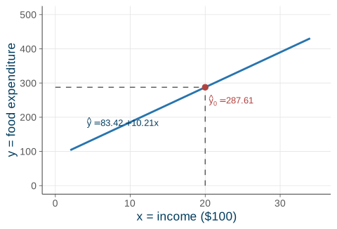
Suppose we want to predict weekly food spending for a household earning $2{,}000 per week, which is $x_0 = 20$ in the units of the data (hundreds of dollars). We plug $x_0$ into the fitted line, \[ \hat y_0 = 83.42 + 10.21(20) = 287.61 . \] Our best single guess for this household’s weekly food spending is $287.61. The arithmetic is identical to “plug $x$ into the line,” but the interpretation is now a forecast for a specific out-of-sample household rather than a fitted value for an in-sample one. Figure 8.1 shows the prediction as the point on the fitted line directly above $x_0 = 20$.

Code

b1 <- 83.42
b2 <- 10.21
x0 <- 20
y0 <- b1 + b2 * x0
line_df <- data.frame(x = seq(2, 34, length.out = 200))
line_df$y <- b1 + b2 * line_df$x
ggplot(line_df, aes(x, y)) +
  geom_line(color = ucla$blue, linewidth = 1) +
  annotate("segment", x = x0, xend = x0, y = 0, yend = y0,
           linetype = "dashed", color = ucla$gray) +
  annotate("segment", x = 0, xend = x0, y = y0, yend = y0,
           linetype = "dashed", color = ucla$gray) +
  annotate("point", x = x0, y = y0, color = ucla$red, size = 2.6) +
  annotate("text", x = x0 + 0.5, y = 250,
           label = "hat(y)[0] == 287.61", parse = TRUE,
           color = ucla$red, hjust = 0, size = 3.4) +
  annotate("text", x = 9, y = 185,
           label = "hat(y) == 83.42 + 10.21 * x", parse = TRUE,
           color = ucla$darkblue, size = 3.4) +
  scale_x_continuous(limits = c(0, 35)) +
  scale_y_continuous(limits = c(0, 500)) +
  labs(x = "x = income ($100)", y = "y = food expenditure")

Figure 8.1: The least squares prediction is the point on the fitted line above $x_0 = 20$, giving $\hat y_0 = 287.61$.

The same prediction is produced by R’s predict() function applied to a new data frame.

predict(fit, newdata = data.frame(income = 20))
#>        1 
#> 287.6089

How good is the prediction?

Because $\hat y_0$ is built from the random estimators $b_1$ and $b_2$, it is itself a random quantity. We judge it through the forecast error, the gap between what actually happens and what we predicted, \[ f = y_0 - \hat y_0 = (\beta_1 + \beta_2 x_0 + e_0) - (b_1 + b_2 x_0). \] Its conditional mean is zero, because $b_1$ and $b_2$ are unbiased and $e_0$ has mean zero, \[ \E(f \given x) = \beta_1 + \beta_2 x_0 + 0 - \bigl[\beta_1 + \beta_2 x_0\bigr] = 0 . \] So $\hat y_0$ is an unbiased predictor. In fact it is the best linear unbiased predictor (BLUP), inheriting that title from $b_1$ and $b_2$ being BLUE.

Unbiased is not pin-point

Unbiasedness does not mean the forecast will be accurate for any single household. The forecast misses for two distinct reasons: we estimated the line (so $b_1, b_2 \neq \beta_1, \beta_2$), and the new household carries its own fresh shock $e_0$ that no model can anticipate. Both sources of error survive even with a perfectly estimated line.

Two predictions, two questions

It pays to be precise about what you are forecasting, because two natural targets share the same point estimate but carry different uncertainty.

The conditional mean $\E(y_0 \given x_0)$

This answers: “What do households at income $x_0$ spend on average?” The only uncertainty comes from estimating the line, so the margin of error is narrower.

The outcome $y_0$

This answers: “What will this particular household spend?” It adds the household’s own shock $e_0$ on top of the estimation error, making it harder to forecast and giving a wider band.

Both targets have the same point estimate, $\hat y_0 = b_1 + b_2 x_0$, but different margins of error. A further warning: prediction is less reliable the farther $x_0$ lies from $\bar x$ — we know the least where we have observed the least, so extrapolating beyond the range of the data is especially risky.

Looking ahead. Quantifying these margins — the prediction interval $\hat y_0 \pm t_c\,\mathrm{se}(f)$ — requires the $t$-distribution and the sum-of-squares decomposition. We return to it in prediction and goodness of fit, once we have inference (confidence intervals and hypothesis testing) in hand.

8.4 Recap

This chapter supplied the last missing piece of the estimation toolkit and put the fitted line to a second use.

Estimating $\sigma^2$. The errors are unobservable, so we use the residuals. Dividing the sum of squared residuals by the degrees of freedom $N - 2$ gives an unbiased estimator, $\hat\sigma^2 = \mathrm{SSE}/(N-2)$. Its square root, the standard error of the regression $\hat\sigma = \sqrt{\hat\sigma^2}$, is the typical vertical miss from the line. For the food data, $\hat\sigma^2 = 8013.3$ and $\hat\sigma = 89.52$.

Standard errors. Substituting $\hat\sigma^2$ into the variance formulas gives estimated variances, whose square roots are the standard errors; for example $\mathrm{se}(b_2) = \sqrt{\hat\sigma^2 / \sum (x_i - \bar x)^2}$. For the food data, $\mathrm{se}(b_1) = 43.41$ and $\mathrm{se}(b_2) = 2.09$. A standard error estimates how much an estimator would vary across repeated samples.

Point prediction. The least squares predictor is the point on the line, $\hat y_0 = b_1 + b_2 x_0$; for the food data at $x_0 = 20$ it gives $\hat y_0 = 287.61$. It is unbiased — indeed the BLUP — with forecast error $f = y_0 - \hat y_0$ satisfying $\E(f \given x) = 0$. Prediction becomes less reliable as $x_0$ moves away from $\bar x$, and forecasting the mean differs from forecasting an individual outcome.

Next time: with estimates and standard errors both in hand, we turn them into a range of plausible values for $\beta_2$ using the $t$-distribution — our first formal act of statistical inference, in confidence intervals.

--- title: "Estimating Error Variance & Prediction" --- {{< include _setup.qmd >}} > **Reading.** SW sec. 4.3, HGL sec. 2.7, 4.1 In the [previous chapter](07-ols-properties.qmd) we showed that OLS is unbiased and, under the Gauss--Markov assumptions, BLUE --- the best linear unbiased estimator. We even wrote down its sampling variance, $$ \Var(b_2 \given x) = \frac{\sigma^2}{\sum (x_i - \bar x)^2}. $$ But every variance and standard error we wrote still hides one unknown: $\sigma^2$, the error variance. Until we can estimate it, those formulas are unusable. This chapter finishes the estimation toolkit. We estimate $\sigma^2$ from the residuals, use it to compute the standard errors of $b_1$ and $b_2$ at last, and then turn the fitted line to a second purpose --- making a point prediction of $y$ at a new value of $x$. After this chapter we have estimates *and* their standard errors: the two ingredients every confidence interval and hypothesis test will need. ## Estimating the error variance {#sec-error-variance} The slope, the intercept, and the error variance are the three unknowns of the simple regression model, and so far we have estimated only the first two. The last one, $\sigma^2$, is what makes precision quantifiable. Under assumption SR2, the errors have conditional mean zero, $\E(e_i \given x) = 0$. The error variance is therefore the average squared error, $$ \sigma^2 = \Var(e_i \given x) = \E(e_i^2 \given x). $$ A variance is an average of squared deviations from the mean, and here the mean is zero, so the natural estimator is just the average squared error, $$ \hat\sigma^2 = \frac{\sum e_i^2}{N}. $$ ::: {.keyidea title="One fatal problem"} The errors $e_i = y_i - \beta_1 - \beta_2 x_i$ are **unobservable** --- computing them requires the unknown $\beta_1$ and $\beta_2$. We can never form $\sum e_i^2$ directly. ::: The fix is the same move we have made all along: replace the unobservable error with its observable stand-in, the **residual**. ### From errors to residuals, with a correction Swap each error $e_i$ for its residual $\hat e_i = y_i - b_1 - b_2 x_i$, which we *can* compute because $b_1$ and $b_2$ are in hand. The obvious candidate is $$ \frac{\sum \hat e_i^2}{N}, $$ but this turns out to be a **biased** estimator of $\sigma^2$. The reason is subtle but important: OLS *chose* $b_1$ and $b_2$ precisely to make $\sum \hat e_i^2$ as small as possible. The residuals are therefore a touch too small on average --- fitting the line to the data uses up some of the variation that the errors would otherwise show. The remedy is a **degrees-of-freedom** correction. ::: {.definition title="Estimator of the error variance"} The unbiased estimator of $\sigma^2$ divides the sum of squared residuals by $N-2$ rather than $N$: $$ \hat\sigma^2 = \frac{\sum_{i=1}^N \hat e_i^2}{N-2} = \frac{\mathrm{SSE}}{N-2}, \qquad\text{and then}\qquad \E(\hat\sigma^2 \given x) = \sigma^2 . $$ Here $\mathrm{SSE} = \sum \hat e_i^2$ is the sum of squared errors (residuals). ::: Why subtract exactly $2$? Because we used the data to estimate $2$ parameters, $\beta_1$ and $\beta_2$, before forming the residuals. Each estimated parameter costs one degree of freedom. The quantity $N-2$ is the **degrees of freedom** of the regression. The same logic explains why the ordinary sample variance of a single variable divides by $N-1$: there you estimate one parameter, the mean, before squaring deviations. ### The standard error of the regression The estimator $\hat\sigma^2$ lives in the *squared* units of $y$, which makes it hard to interpret directly. Taking its square root returns us to the units of $y$ and gives a quantity with its own name. ::: {.definition title="Standard error of the regression (SER)"} $$ \hat\sigma = \sqrt{\hat\sigma^2} $$ is the **standard error of the regression** --- the typical vertical distance of a data point from the fitted line. ::: ::: {.keyidea title="How to read the SER"} $\hat\sigma$ measures the **typical vertical distance** of a data point from the fitted line --- the size of a typical residual, in the units of the dependent variable. A small SER means the points hug the line; a large SER means a loose scatter that the regression explains only partially. ::: ::: {.callout-note appearance="simple"} **Naming.** Software labels this quantity in many ways: "S.E. of regression" (EViews), "Residual standard error" (R), "Root MSE" (Stata). They are all the same number, $\hat\sigma$. ::: ### Worked example: the food data Return to the food-expenditure data (HGL Example 2.5), where the fitted line is $\hat y = 83.42 + 10.21\,x$ with $x$ measured in hundreds of dollars of weekly income. To estimate $\sigma^2$ we sum the $40$ squared residuals, $$ \mathrm{SSE} = \sum \hat e_i^2 = 304{,}505.2 , $$ then divide by the degrees of freedom $N - 2 = 38$: $$ \hat\sigma^2 = \frac{304{,}505.2}{38} = 8013.29, \qquad \hat\sigma = \sqrt{8013.29} = 89.52 . $$ A *typical* household sits about \$89.52 above or below the fitted line. That is a large spread relative to the predicted spending levels, a reminder that income alone leaves a great deal of food-expenditure variation unexplained. The residuals for the first five households illustrate the raw material of this calculation; each is the gap between actual spending $y$ and the fitted value $\hat y = 83.42 + 10.21\,x$. ```{r} #| label: tbl-residuals #| tbl-cap: "Residuals for the first five households, using $\\hat y = 83.42 + 10.21\\,x$." res_tab <- data.frame( x = c(3.69, 4.39, 4.75, 6.03, 12.47), y = c(115.22, 135.98, 119.34, 114.96, 187.05), yhat = c(121.09, 128.24, 131.91, 144.98, 210.73), ehat = c(-5.87, 7.74, -12.57, -30.02, -23.68) ) knitr::kable( res_tab, col.names = c("$x$", "$y$", "$\\hat y$", "$\\hat e = y - \\hat y$"), align = "rrrr" ) ``` In R this entire calculation is a single line. The residual standard error reported by `summary()` *is* the SER, and `sum(resid(fit)^2)` is the SSE. ```{r} #| code-fold: false data(food) fit <- lm(food_exp ~ income, data = food) sse <- sum(resid(fit)^2) # SSE = sum of squared residuals N <- nrow(food) sig2 <- sse / (N - 2) # sigma-hat squared c(SSE = sse, sigma2_hat = sig2, SER = sqrt(sig2)) ``` ```{r} #| code-fold: false summary(fit)$sigma # the SER, labeled "Residual standard error" ``` ## Standard errors at last {#sec-standard-errors} With an estimate of $\sigma^2$ in hand, the variance formulas from the previous chapter finally become computable. In [Chapter 7](07-ols-properties.qmd) each of those formulas contained the unknown $\sigma^2$; replacing it with $\hat\sigma^2$ turns the *true* variances into *estimated* variances. ::: {.definition title="Estimated variances and covariance of the OLS estimators"} $$ \widehat{\Var}(b_2 \given x) = \frac{\hat\sigma^2}{\sum (x_i - \bar x)^2}, \qquad \widehat{\Var}(b_1 \given x) = \hat\sigma^2 \!\left[\frac{\sum x_i^2}{N \sum (x_i - \bar x)^2}\right], $$ $$ \widehat{\Cov}(b_1, b_2 \given x) = \hat\sigma^2 \!\left[\frac{-\bar x}{\sum (x_i - \bar x)^2}\right]. $$ The **standard errors** are the square roots of the estimated variances, $$ \mathrm{se}(b_1) = \sqrt{\widehat{\Var}(b_1 \given x)}, \qquad \mathrm{se}(b_2) = \sqrt{\widehat{\Var}(b_2 \given x)} . $$ ::: ### The variance--covariance matrix Software collects these three estimated quantities --- the two variances and the covariance --- into a single $2 \times 2$ array called the **variance--covariance matrix**. Its diagonal holds the variances and its off-diagonal entries hold the covariance: $$ \begin{bmatrix} \widehat{\Var}(b_1) & \widehat{\Cov}(b_1, b_2)\\[2pt] \widehat{\Cov}(b_1, b_2) & \widehat{\Var}(b_2) \end{bmatrix} = \begin{bmatrix} 1884.44 & -85.90\\[2pt] -85.90 & 4.3818 \end{bmatrix} . $$ Square-rooting the diagonal gives the standard errors for the food data, $$ \mathrm{se}(b_1) = \sqrt{1884.44} = 43.41, \qquad \mathrm{se}(b_2) = \sqrt{4.3818} = 2.09 . $$ ::: {.keyidea title="Does it pass a sanity check?"} Across the $10$ hypothetical samples studied in [Chapter 7](07-ols-properties.qmd), the estimates $b_2$ had a standard deviation of $1.58$. Our standard error computed from a **single** sample, $2.09$, is in the same ballpark. That is reassuring: a standard error really is an estimate of the sample-to-sample spread of an estimator across repeated samples. ::: In R the variance--covariance matrix is returned by `vcov()`, and the standard errors are the square roots of its diagonal. ```{r} #| code-fold: false vcov(fit) # the estimated variance-covariance matrix sqrt(diag(vcov(fit))) # the standard errors of b1 and b2 ``` ### Reporting a fitted regression Now that estimates travel with standard errors, we can adopt the compact reporting convention used throughout applied econometrics (HGL Example 4.3): the standard error appears in parentheses directly beneath each coefficient, with the SER reported alongside, $$ \widehat{\text{FOOD\_EXP}} = \underset{(43.41)}{83.42} + \underset{(2.09)}{10.21}\,\text{INCOME}, \qquad \hat\sigma = 89.52 . $$ Why report standard errors rather than just the point estimates? Because they let any reader immediately do three things. First, they gauge **precision**: a small standard error means a sharply estimated coefficient. Second, they support a quick interval estimate --- roughly $b_k \pm 2\,\mathrm{se}(b_k)$ when $N - 2 > 30$, which we make precise with the $t$-distribution in [the next chapter](09-confidence-intervals.qmd). Third, they allow hypothesis tests; for example, to test $H_0 : \beta_2 = 8$ we would form $t = (10.21 - 8)/2.09$, a calculation we develop in [hypothesis testing](10-hypothesis-testing.qmd). Estimates without standard errors are nearly useless. ## Point prediction {#sec-prediction} The fitted line has a second use beyond describing the sample at hand: it can **forecast** $y$ for a household that is not in the sample. Suppose a new household has income $x_0$. By assumption SR1 it obeys the same model as every other, $$ y_0 = \beta_1 + \beta_2 x_0 + e_0, \qquad \E(e_0) = 0 . $$ The key is to split the outcome into a part we can estimate and a part we cannot, $$ y_0 = \underbrace{\beta_1 + \beta_2 x_0}_{\text{estimate this}} + \underbrace{e_0}_{\text{best guess } 0} . $$ We estimate the systematic part by $b_1 + b_2 x_0$, and we predict the random shock $e_0$ by its mean, which is zero. Putting the two together gives the forecast. ::: {.definition title="Least squares predictor"} The **least squares predictor** of $y$ at a new value $x_0$ is the point on the fitted line, $$ \hat y_0 = b_1 + b_2 x_0 . $$ ::: ### Worked example: predicting at a new income Suppose we want to predict weekly food spending for a household earning \$2{,}000 per week, which is $x_0 = 20$ in the units of the data (hundreds of dollars). We plug $x_0$ into the fitted line, $$ \hat y_0 = 83.42 + 10.21(20) = 287.61 . $$ Our best single guess for this household's weekly food spending is \$287.61. The arithmetic is identical to "plug $x$ into the line," but the interpretation is now a forecast for a specific out-of-sample household rather than a fitted value for an in-sample one. @fig-prediction shows the prediction as the point on the fitted line directly above $x_0 = 20$. ```{r} #| label: fig-prediction #| fig-cap: "The least squares prediction is the point on the fitted line above $x_0 = 20$, giving $\\hat y_0 = 287.61$." #| fig-width: 5 #| fig-height: 3.4 b1 <- 83.42 b2 <- 10.21 x0 <- 20 y0 <- b1 + b2 * x0 line_df <- data.frame(x = seq(2, 34, length.out = 200)) line_df$y <- b1 + b2 * line_df$x ggplot(line_df, aes(x, y)) + geom_line(color = ucla$blue, linewidth = 1) + annotate("segment", x = x0, xend = x0, y = 0, yend = y0, linetype = "dashed", color = ucla$gray) + annotate("segment", x = 0, xend = x0, y = y0, yend = y0, linetype = "dashed", color = ucla$gray) + annotate("point", x = x0, y = y0, color = ucla$red, size = 2.6) + annotate("text", x = x0 + 0.5, y = 250, label = "hat(y)[0] == 287.61", parse = TRUE, color = ucla$red, hjust = 0, size = 3.4) + annotate("text", x = 9, y = 185, label = "hat(y) == 83.42 + 10.21 * x", parse = TRUE, color = ucla$darkblue, size = 3.4) + scale_x_continuous(limits = c(0, 35)) + scale_y_continuous(limits = c(0, 500)) + labs(x = "x = income ($100)", y = "y = food expenditure") ``` The same prediction is produced by R's `predict()` function applied to a new data frame. ```{r} #| code-fold: false predict(fit, newdata = data.frame(income = 20)) ``` ### How good is the prediction? Because $\hat y_0$ is built from the random estimators $b_1$ and $b_2$, it is itself a random quantity. We judge it through the **forecast error**, the gap between what actually happens and what we predicted, $$ f = y_0 - \hat y_0 = (\beta_1 + \beta_2 x_0 + e_0) - (b_1 + b_2 x_0). $$ Its conditional mean is zero, because $b_1$ and $b_2$ are unbiased and $e_0$ has mean zero, $$ \E(f \given x) = \beta_1 + \beta_2 x_0 + 0 - \bigl[\beta_1 + \beta_2 x_0\bigr] = 0 . $$ So $\hat y_0$ is an **unbiased predictor**. In fact it is the **best linear unbiased predictor (BLUP)**, inheriting that title from $b_1$ and $b_2$ being BLUE. ::: {.warningbox title="Unbiased is not pin-point"} Unbiasedness does **not** mean the forecast will be accurate for any single household. The forecast misses for **two** distinct reasons: we estimated the line (so $b_1, b_2 \neq \beta_1, \beta_2$), and the new household carries its own fresh shock $e_0$ that no model can anticipate. Both sources of error survive even with a perfectly estimated line. ::: ### Two predictions, two questions It pays to be precise about *what* you are forecasting, because two natural targets share the same point estimate but carry different uncertainty. ::: {.keyidea title="The conditional mean $\\E(y_0 \\given x_0)$"} This answers: "What do households at income $x_0$ spend **on average**?" The only uncertainty comes from estimating the line, so the margin of error is narrower. ::: ::: {.keyidea title="The outcome $y_0$"} This answers: "What will **this particular** household spend?" It adds the household's own shock $e_0$ on top of the estimation error, making it **harder** to forecast and giving a wider band. ::: Both targets have the same point estimate, $\hat y_0 = b_1 + b_2 x_0$, but *different* margins of error. A further warning: prediction is **less reliable the farther $x_0$ lies from $\bar x$** --- we know the least where we have observed the least, so extrapolating beyond the range of the data is especially risky. ::: {.callout-note appearance="simple"} **Looking ahead.** Quantifying these margins --- the **prediction interval** $\hat y_0 \pm t_c\,\mathrm{se}(f)$ --- requires the $t$-distribution and the sum-of-squares decomposition. We return to it in [prediction and goodness of fit](11-prediction-fit.qmd), once we have inference ([confidence intervals](09-confidence-intervals.qmd) and [hypothesis testing](10-hypothesis-testing.qmd)) in hand. ::: ## Recap {#sec-recap} This chapter supplied the last missing piece of the estimation toolkit and put the fitted line to a second use. **Estimating $\sigma^2$.** The errors are unobservable, so we use the residuals. Dividing the sum of squared residuals by the degrees of freedom $N - 2$ gives an unbiased estimator, $\hat\sigma^2 = \mathrm{SSE}/(N-2)$. Its square root, the standard error of the regression $\hat\sigma = \sqrt{\hat\sigma^2}$, is the typical vertical miss from the line. For the food data, $\hat\sigma^2 = 8013.3$ and $\hat\sigma = 89.52$. **Standard errors.** Substituting $\hat\sigma^2$ into the variance formulas gives estimated variances, whose square roots are the standard errors; for example $\mathrm{se}(b_2) = \sqrt{\hat\sigma^2 / \sum (x_i - \bar x)^2}$. For the food data, $\mathrm{se}(b_1) = 43.41$ and $\mathrm{se}(b_2) = 2.09$. A standard error estimates how much an estimator would vary across repeated samples. **Point prediction.** The least squares predictor is the point on the line, $\hat y_0 = b_1 + b_2 x_0$; for the food data at $x_0 = 20$ it gives $\hat y_0 = 287.61$. It is unbiased --- indeed the BLUP --- with forecast error $f = y_0 - \hat y_0$ satisfying $\E(f \given x) = 0$. Prediction becomes less reliable as $x_0$ moves away from $\bar x$, and forecasting the mean differs from forecasting an individual outcome. **Next time:** with estimates and standard errors both in hand, we turn them into a range of plausible values for $\beta_2$ using the $t$-distribution --- our first formal act of statistical inference, in [confidence intervals](09-confidence-intervals.qmd).