In the last chapter we fit the line. The least-squares formulas \(b_2 = \widehat{\Cov}(x,y)/\widehat{\Var}(x)\) and \(b_1 = \bar y - b_2\bar x\) turned the food-expenditure data into \[
\widehat{\text{FOOD\_EXP}} = 83.42 + 10.21\,\text{INCOME}.
\] The natural next question is: how good is this estimate? HGL’s answer is blunt — that question is unanswerable. We will never observe \(\beta_2\), so we can never say how close \(10.21\) lands to it.
So we change the question. Instead of judging a single estimate, we judge the estimation procedure — the random variables \(b_1\) and \(b_2\) that the procedure produces. This chapter shows that OLS is unbiased (on average across samples it nails \(\beta\)), works out its variance (its precision) and what drives it, and closes with the Gauss–Markov theorem: under the standard assumptions OLS is BLUE, the Best Linear Unbiased Estimator. The remaining unknown, \(\sigma^2\), and the standard errors that depend on it are the subject of the next chapter.
7.1 The estimator as a random variable
Draw another 40 households — the same incomes, but new families — and you get different estimates, because each \(y_i\) is random. HGL report ten hypothetical samples drawn from the same population, and the slopes wander all over the place.
Table 7.1: Ten hypothetical samples from one population. The same procedure gives different numbers each time.
sample
\(b_1\)
\(b_2\)
1
93.64
8.24
2
91.62
8.90
3
126.76
6.59
4
55.98
11.23
\(\vdots\)
\(\vdots\)
\(\vdots\)
10
128.55
6.99
avg
96.11
8.70
Across these samples \(b_2\) ranges from \(6.59\) to \(11.23\): the same procedure applied to different data produces different numbers. This sampling variation is unavoidable — \(b_1\) and \(b_2\) are random variables with a distribution. A hopeful sign is that the average slope across the ten samples, \(8.70\), sits near the truth, hinting at unbiasedness. With a single sample we can never see this spread directly, so we study it theoretically instead.
OLS is a linear estimator
To study the distribution of \(b_2\), we first rewrite it in a more revealing form (HGL Appendix 2C). Starting from the deviation form of the slope and using \(\sum (x_i - \bar x)\bar y = 0\), the estimator collapses to a weighted average of the \(y_i\): \[
b_2 = \sum_{i=1}^N w_i\, y_i,
\qquad
w_i = \frac{x_i - \bar x}{\sum_{j}(x_j-\bar x)^2}.
\]
The weights \(w_i\) depend only on \(x\). Once we condition on the regressor, they are simply constants. This puts OLS into an important category.
Linear estimator
An estimator is a linear estimator if it is a weighted average of the \(y_i\), \(\sum_i w_i y_i\), with weights that do not depend on the \(y_i\). OLS is a linear estimator — a fact we will lean on heavily when we get to Gauss–Markov.
Two facts that do all the bookkeeping. The OLS weights satisfy \(\sum_i w_i = 0\) and \(\sum_i w_i x_i = 1\). These two identities appear in every proof below.
The key decomposition
Now substitute the model \(y_i = \beta_1 + \beta_2 x_i + e_i\) into \(b_2 = \sum w_i y_i\) and apply \(\sum w_i = 0\) and \(\sum w_i x_i = 1\). The intercept and slope terms collapse, leaving the single most important equation of the chapter: \[
b_2 = \beta_2 + \sum_{i=1}^N w_i\, e_i .
\]
The workhorse decomposition
\[
b_2 = \underbrace{\beta_2}_{\text{what we want (fixed)}}
\;+\;
\underbrace{\sum_i w_i e_i}_{\text{estimation error (random)}}.
\] Everything random about \(b_2\) lives in the error term \(\sum_i w_i e_i\). Its mean controls bias; its variance controls precision. We take them in turn.
7.2 Unbiasedness
Take the conditional expectation of the decomposition \(b_2 = \beta_2 + \sum w_i e_i\) given \(x\): \[
\begin{aligned}
\E(b_2 \given x)
&= \beta_2 + \sum_i w_i\,\E(e_i \given x)\\
&= \beta_2 + \sum_i w_i \cdot 0
= \beta_2 .
\end{aligned}
\] Two ingredients make this work. First, each \(w_i\) is constant given \(x\), so it pulls straight out of the expectation. Second, assumption SR2 says \(\E(e_i \given x) = 0\), which zeroes out the entire error term.
Unbiasedness of OLS
An estimator is unbiased if its expected value equals the parameter it estimates. Under assumptions SR1–SR5, \[
\E(b_2 \given x) = \beta_2
\qquad\text{and}\qquad
\E(b_1 \given x) = \beta_1 .
\]
What unbiasedness does and does not say
It is worth being precise about the claim, because it is easy to over-read.
Unbiasedness does say that, over all possible samples, the estimates average out to the true \(\beta_2\). The procedure is centered on the target — no systematic over- or under-shooting.
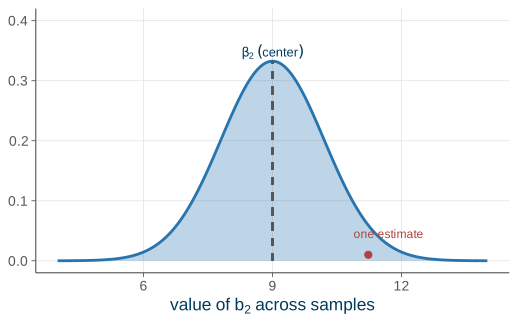
Unbiasedness does not say that your particular estimate, \(10.21\), is close to \(\beta_2\). A single draw can land far from the center of the distribution. Unbiasedness is a property of the estimator (the procedure), never of a single estimate.
Figure 7.1 makes the distinction visual. The bell curve is the sampling distribution of \(b_2\), centered exactly on \(\beta_2\). Any one sample gives a single draw from that curve — and that draw can sit well off-center even though the curve as a whole is correctly centered.
Code
xs<-seq(4, 14, length.out =400)dat<-data.frame(x =xs, y =dnorm(xs, mean =9, sd =1.2))ggplot(dat, aes(x, y))+geom_area(fill =ucla$blue, alpha =0.30)+geom_line(color =ucla$blue, linewidth =1)+geom_segment(aes(x =9, xend =9, y =0, yend =dnorm(9, 9, 1.2)), linetype ="dashed", color =ucla$gray)+annotate("text", x =9, y =dnorm(9, 9, 1.2)+0.015, label ="beta[2]~(center)", parse =TRUE, color =ucla$darkblue, size =3.4)+annotate("point", x =11.23, y =0.01, color =ucla$red, size =2.2)+annotate("text", x =11.7, y =0.045, label ="one estimate", color =ucla$red, size =3.2)+scale_y_continuous(limits =c(0, 0.40))+labs(x =expression(value~of~b[2]~across~samples), y =NULL)
Figure 7.1: The sampling distribution of \(b_2\) is centered on \(\beta_2\), but any one estimate can land far from the center.
When unbiasedness fails: omitted variables
The entire proof leaned on SR2, \(\E(e_i \given x) = 0\). If that assumption breaks, so does unbiasedness: \[
\E(e_i \given x) \neq 0
\;\Longrightarrow\;
\E(b_2 \given x) = \beta_2 + \sum_i w_i\,\E(e_i \given x) \neq \beta_2 .
\]
The classic way SR2 fails is when a variable that belongs in the model has been left out and lurks in the error term.
Omitting ability from a wage equation
Consider \(\text{WAGE} = \beta_1 + \beta_2\,\text{EDUC} + e\), with a worker’s ability buried inside \(e\). Ability is correlated with education, so \(\E(e \given \text{EDUC}) \neq 0\). As a result \(b_2\) is biased: it confounds the genuine return to schooling with the payoff to ability.
This is omitted-variable bias — the formal face of the slogan “correlation \(\neq\) causation.” We quantify it precisely when we get to model specification.
7.3 Variance and precision
Being unbiased is not enough on its own. We want estimates that are tightly clustered around \(\beta\), not merely centered on it. That tightness is the variance of the estimator. Under assumptions SR1–SR5 (HGL Appendix 2E), the variances and covariance of the OLS estimators are \[
\Var(b_2 \given x) = \frac{\sigma^2}{\sum (x_i-\bar x)^2},
\qquad
\Var(b_1 \given x) = \sigma^2\!\left[\frac{\sum x_i^2}{N\sum(x_i-\bar x)^2}\right],
\]\[
\Cov(b_1, b_2 \given x) = \sigma^2\!\left[\frac{-\bar x}{\sum(x_i-\bar x)^2}\right].
\]
Smaller variance means more precise
Take two unbiased estimators with the same center. Prefer the one with the smaller variance — it has a higher chance of landing near \(\beta_2\) on any given sample. Most of what follows is about \(\Var(b_2 \given x)\).
What drives the precision of \(b_2\)?
Look hard at \(\displaystyle \Var(b_2 \given x) = \frac{\sigma^2}{\sum(x_i-\bar x)^2}\). Three levers control it.
Error variance \(\sigma^2\) (the numerator). Noisier data about the line means a less precise slope. We cannot control this — it is a feature of the population.
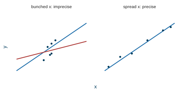
Spread of \(x\), measured by \(\sum(x_i-\bar x)^2\) (the denominator). More variation in income means a more precise slope. A wide lever arm pins the line down firmly.
Sample size \(N\). Each additional observation adds a term to the denominator sum, so a larger \(N\) shrinks the variance: more data, tighter estimates.
The second lever is the easiest to picture. Figure 7.2 contrasts a sample with bunched-up \(x\) values against one with spread-out \(x\) values. When the \(x\)’s are bunched together, very different lines fit the cloud about equally well, so the slope is poorly determined. Spread the same number of points across a wide range of \(x\) and the line is nailed down.
Code
bunched<-data.frame( x =c(4, 4.5, 5, 5.5, 5, 4.8), y =c(3, 5, 4, 6, 5.5, 3.8), panel ="bunched x: imprecise")spread<-data.frame( x =c(1, 2.5, 4, 6, 8, 9), y =c(2, 3.5, 4, 6, 7.5, 8), panel ="spread x: precise")pts<-rbind(bunched, spread)fits<-data.frame( x =c(0.5, 9.5, 0.5, 9.5, 0.5, 9.5), y =c(1+0.8*0.5, 1+0.8*9.5, # line 1, bunched3+0.3*0.5, 3+0.3*9.5, # line 2, bunched1+0.8*0.5, 1+0.8*9.5), # line 1, spread grp =c("a", "a", "b", "b", "c", "c"), panel =c("bunched x: imprecise", "bunched x: imprecise","bunched x: imprecise", "bunched x: imprecise","spread x: precise", "spread x: precise"))ggplot()+geom_line(data =fits, aes(x, y, group =grp, color =grp), linewidth =1)+geom_point(data =pts, aes(x, y), color =ucla$darkblue, size =1.6)+scale_color_manual(values =c(a =ucla$blue, b =ucla$red, c =ucla$blue), guide ="none")+facet_wrap(~panel)+scale_x_continuous(limits =c(0, 10), breaks =NULL)+scale_y_continuous(limits =c(0, 10), breaks =NULL)+labs(x ="x", y ="y")
Figure 7.2: Bunched regressors (left) leave the slope poorly determined; spread-out regressors (right) pin it down.
From variance to standard error
There is a catch: every variance formula above contains the unknown error variance \(\sigma^2\). To make them operational we replace \(\sigma^2\) with an estimate \(\hat\sigma^2\) (the subject of the next chapter). This gives an estimated variance, and its square root is the standard error: \[
\mathrm{se}(b_2) = \sqrt{\widehat{\Var}(b_2 \given x)}
= \sqrt{\frac{\hat\sigma^2}{\sum(x_i-\bar x)^2}} .
\]
The standard error is our estimate of the sampling standard deviation of \(b_2\) — it answers “how far, typically, would \(b_2\) land from \(\beta_2\) across samples?” For the food-expenditure data, software reports \(\mathrm{se}(b_1) = 43.41\) and \(\mathrm{se}(b_2) = 2.09\). We can read both straight off the standard lm() output:
data(food)fit<-lm(food_exp~income, data =food)summary(fit)$coefficients#> Estimate Std. Error t value Pr(>|t|)#> (Intercept) 83.41600 43.410163 1.921578 6.218242e-02#> income 10.20964 2.093264 4.877381 1.945862e-05
The Std. Error column reproduces the slide’s numbers. Standard errors are the raw material of every confidence interval and \(t\)-test to come (see confidence intervals and hypothesis testing). But to actually compute them we first need \(\hat\sigma^2\) — that is the first order of business next chapter.
The shape of the distribution
The center (\(\beta_2\)) and the spread (\(\Var(b_2 \given x)\)) describe where the sampling distribution sits and how wide it is. What about its shape? The answer depends on whether the errors are normal.
If SR6 holds: exactly normal
If the errors are normally distributed, then \(b_2 = \sum w_i y_i\) is a weighted sum of normal random variables, hence exactly normal: \[
b_2 \given x \sim N\!\left(\beta_2,\ \frac{\sigma^2}{\sum(x_i-\bar x)^2}\right).
\]
If SR6 fails: a central limit theorem
Even with non-normal errors, \(b_2\) is approximately normal in large samples. Because \(b_2\) is essentially an average (a weighted sum of the \(y_i\)), a central limit theorem applies.
Either way — exactly under normality, or approximately in large samples — \(b_2\) ends up normal. That normal shape is precisely what makes the \(t\)-based inference of the next several chapters possible.
7.4 The Gauss–Markov theorem
We now know two things about OLS: it is linear (\(b_2 = \sum w_i y_i\)) and it is unbiased (\(\E(b_2 \given x) = \beta_2\)). The remaining question is whether it is the best such estimator. The answer is the central theoretical result of the simple regression model.
Gauss--Markov theorem
Given \(x\) and under assumptions SR1–SR5, the OLS estimators \(b_1\) and \(b_2\) have the smallest variance among all linear and unbiased estimators of \(\beta_1\) and \(\beta_2\). OLS is the Best Linear Unbiased Estimator (BLUE).
In words: within the class of estimators that are (i) weighted averages of the \(y_i\) and (ii) correct on average, nothing beats OLS on precision. There is no point hunting for a cleverer linear unbiased rule — you already hold the winner.
Reading the fine print
Gauss–Markov is precise about exactly what it promises, and each qualifier matters.
“Best” is only within a class — linear and unbiased. A nonlinear or biased estimator could, in principle, have a smaller variance.
“Best” means minimum variance among that class.
It requires SR1–SR5. Break any one of them — for instance, heteroskedasticity breaks SR3 — and OLS need no longer be best.
It does not need normality (SR6). Gauss–Markov is a pure first- and second-moment result; it says nothing about the shape of the distribution.
It applies to the estimators, the procedure — not to the estimates from any single sample.
Stock & Watson call the same result the Gauss–Markov theorem too (sec. 5.5). Their efficiency statement is the textbook’s reason OLS is the default estimator almost everywhere in applied work.
What each assumption buys you
It helps to keep a scorecard of which property leans on which assumption. Each result in this chapter needs only some of the assumptions, and much of the rest of econometrics is a tour of which assumption is failing and what to do about it.
Table 7.2: Which OLS property each assumption buys.
Property
Needs
Why
\(b_1, b_2\) exist / computable
SR1, SR5
line defined; \(\sum(x_i-\bar x)^2 \neq 0\)
Unbiased: \(\E(b\mid x)=\beta\)
SR1, SR2
\(\E(e\mid x)=0\) kills the bias term
Variance formulas as stated
SR1–SR4
SR3 (homoskedasticity), SR4 (uncorrelated)
BLUE (Gauss–Markov)
SR1–SR5
minimum variance in class
Exact normal \(b\), exact inference
+ SR6
normal errors \(\Rightarrow\) normal \(b\)
When an assumption fails there is usually a standard remedy: robust standard errors when SR3 (homoskedasticity) breaks, clustering when SR4 (uncorrelated errors) breaks, and instrumental variables when SR2 (exogeneity) breaks. The chapters ahead work through these one at a time.
7.5 Recap
The estimate \(10.21\) is one draw of a random estimator, so we judge the procedure, not the number.
The estimator is random. OLS is a linear estimator, \(b_2 = \sum_i w_i y_i\) with \(w_i = (x_i - \bar x)/\sum_j(x_j-\bar x)^2\), and it decomposes as \(b_2 = \beta_2 + \sum_i w_i e_i\) — the second term holds all the randomness.
Unbiased.\(\E(b_2 \given x) = \beta_2\) (it needs SR2), a statement about the procedure rather than any single estimate. It fails under omitted variables.
Precision.\(\Var(b_2 \given x) = \sigma^2 / \sum(x_i-\bar x)^2\) is smaller when \(\sigma^2\) is low, when \(x\) is spread out, and when \(N\) is large. The standard error is \(\mathrm{se}(b_2) = \sqrt{\hat\sigma^2/\sum(x_i-\bar x)^2}\).
Gauss–Markov. Under SR1–SR5, OLS is BLUE. Normality (SR6) is optional and is needed only for an exactly normal \(b\).
Next time: the last remaining unknown, \(\sigma^2\). We estimate it with \(\hat\sigma^2 = \mathrm{SSE}/(N-2)\), build the standard error of the regression on top of it, and use the fitted line to make point predictions — variance estimation and prediction.
Source Code
---title: "Properties of OLS & the Gauss--Markov Theorem"---{{< include _setup.qmd >}}> **Reading.** SW sec. 4.5, 5.5, HGL sec. 2.4--2.6In the [last chapter](06-ols-estimation.qmd) we fit the line. The least-squaresformulas $b_2 = \widehat{\Cov}(x,y)/\widehat{\Var}(x)$ and $b_1 = \bar y - b_2\bar x$turned the food-expenditure data into$$\widehat{\text{FOOD\_EXP}} = 83.42 + 10.21\,\text{INCOME}.$$The natural next question is: **how good is this estimate?** HGL's answer isblunt --- that question is *unanswerable*. We will never observe $\beta_2$, so wecan never say how close $10.21$ lands to it.So we change the question. Instead of judging a single estimate, we judge the**estimation procedure** --- the random variables $b_1$ and $b_2$ that theprocedure produces. This chapter shows that OLS is **unbiased** (on averageacross samples it nails $\beta$), works out its **variance** (its precision) andwhat drives it, and closes with the **Gauss--Markov theorem**: under the standardassumptions OLS is *BLUE*, the Best Linear Unbiased Estimator. The remainingunknown, $\sigma^2$, and the standard errors that depend on it are the subject of[the next chapter](08-variance-prediction.qmd).## The estimator as a random variable {#sec-random-estimator}Draw another 40 households --- the same incomes, but new families --- and you get*different* estimates, because each $y_i$ is random. HGL report ten hypotheticalsamples drawn from the *same* population, and the slopes wander all over theplace.```{r}#| label: tbl-samples#| tbl-cap: "Ten hypothetical samples from one population. The same procedure gives different numbers each time."samples <-data.frame(sample =c("1", "2", "3", "4", "$\\vdots$", "10", "**avg**"),b1 =c("93.64", "91.62", "126.76", "55.98", "$\\vdots$", "128.55", "**96.11**"),b2 =c("8.24", "8.90", "6.59", "11.23", "$\\vdots$", "6.99", "**8.70**"))knitr::kable(samples, col.names =c("sample", "$b_1$", "$b_2$"), align ="ccc")```Across these samples $b_2$ ranges from $6.59$ to $11.23$: the same procedureapplied to different data produces different numbers. This **sampling variation**is unavoidable --- $b_1$ and $b_2$ are **random variables** with a distribution. Ahopeful sign is that the average slope across the ten samples, $8.70$, sits nearthe truth, hinting at unbiasedness. With a single sample we can never see thisspread directly, so we study it *theoretically* instead.### OLS is a linear estimatorTo study the distribution of $b_2$, we first rewrite it in a more revealingform (HGL Appendix 2C). Starting from the deviation form of the slope and using$\sum (x_i - \bar x)\bar y = 0$, the estimator collapses to a weighted average ofthe $y_i$:$$b_2 = \sum_{i=1}^N w_i\, y_i,\qquadw_i = \frac{x_i - \bar x}{\sum_{j}(x_j-\bar x)^2}.$$The weights $w_i$ depend **only on $x$**. Once we condition on the regressor,they are simply constants. This puts OLS into an important category.::: {.definition title="Linear estimator"}An estimator is a **linear estimator** if it is a weighted average of the$y_i$, $\sum_i w_i y_i$, with weights that do not depend on the $y_i$. OLS is alinear estimator --- a fact we will lean on heavily when we get toGauss--Markov.:::::: {.callout-note appearance="simple"}**Two facts that do all the bookkeeping.** The OLS weights satisfy$\sum_i w_i = 0$ and $\sum_i w_i x_i = 1$. These two identities appear in everyproof below.:::### The key decompositionNow substitute the model $y_i = \beta_1 + \beta_2 x_i + e_i$ into$b_2 = \sum w_i y_i$ and apply $\sum w_i = 0$ and $\sum w_i x_i = 1$. Theintercept and slope terms collapse, leaving the single most important equation ofthe chapter:$$b_2 = \beta_2 + \sum_{i=1}^N w_i\, e_i .$$::: {.keyidea title="The workhorse decomposition"}$$b_2 = \underbrace{\beta_2}_{\text{what we want (fixed)}}\;+\;\underbrace{\sum_i w_i e_i}_{\text{estimation error (random)}}.$$Everything random about $b_2$ lives in the error term $\sum_i w_i e_i$. Its**mean** controls bias; its **variance** controls precision. We take them inturn.:::## Unbiasedness {#sec-unbiasedness}Take the conditional expectation of the decomposition $b_2 = \beta_2 + \sum w_i e_i$given $x$:$$\begin{aligned}\E(b_2 \given x) &= \beta_2 + \sum_i w_i\,\E(e_i \given x)\\ &= \beta_2 + \sum_i w_i \cdot 0 = \beta_2 .\end{aligned}$$Two ingredients make this work. First, each $w_i$ is constant given $x$, so itpulls straight out of the expectation. Second, assumption **SR2** says$\E(e_i \given x) = 0$, which zeroes out the entire error term.::: {.property title="Unbiasedness of OLS"}An estimator is **unbiased** if its expected value equals the parameter itestimates. Under assumptions SR1--SR5,$$\E(b_2 \given x) = \beta_2\qquad\text{and}\qquad\E(b_1 \given x) = \beta_1 .$$:::### What unbiasedness does and does not sayIt is worth being precise about the claim, because it is easy to over-read.Unbiasedness **does** say that, over *all possible samples*, the estimatesaverage out to the true $\beta_2$. The procedure is centered on the target --- nosystematic over- or under-shooting.Unbiasedness **does not** say that *your* particular estimate, $10.21$, is closeto $\beta_2$. A single draw can land far from the center of the distribution.Unbiasedness is a property of the **estimator** (the procedure), never of asingle **estimate**.@fig-sampling makes the distinction visual. The bell curve is the samplingdistribution of $b_2$, centered exactly on $\beta_2$. Any one sample gives asingle draw from that curve --- and that draw can sit well off-center even thoughthe curve as a whole is correctly centered.```{r}#| label: fig-sampling#| fig-cap: "The sampling distribution of $b_2$ is centered on $\\beta_2$, but any one estimate can land far from the center."#| fig-width: 5.4#| fig-height: 3.4xs <-seq(4, 14, length.out =400)dat <-data.frame(x = xs, y =dnorm(xs, mean =9, sd =1.2))ggplot(dat, aes(x, y)) +geom_area(fill = ucla$blue, alpha =0.30) +geom_line(color = ucla$blue, linewidth =1) +geom_segment(aes(x =9, xend =9, y =0, yend =dnorm(9, 9, 1.2)),linetype ="dashed", color = ucla$gray) +annotate("text", x =9, y =dnorm(9, 9, 1.2) +0.015,label ="beta[2]~(center)", parse =TRUE, color = ucla$darkblue,size =3.4) +annotate("point", x =11.23, y =0.01, color = ucla$red, size =2.2) +annotate("text", x =11.7, y =0.045, label ="one estimate",color = ucla$red, size =3.2) +scale_y_continuous(limits =c(0, 0.40)) +labs(x =expression(value~of~b[2]~across~samples), y =NULL)```### When unbiasedness fails: omitted variablesThe entire proof leaned on **SR2**, $\E(e_i \given x) = 0$. If that assumptionbreaks, so does unbiasedness:$$\E(e_i \given x) \neq 0\;\Longrightarrow\;\E(b_2 \given x) = \beta_2 + \sum_i w_i\,\E(e_i \given x) \neq \beta_2 .$$The classic way SR2 fails is when a variable that belongs in the model has beenleft out and lurks in the error term.::: {.example title="Omitting ability from a wage equation"}Consider $\text{WAGE} = \beta_1 + \beta_2\,\text{EDUC} + e$, with a worker's*ability* buried inside $e$. Ability is correlated with education, so$\E(e \given \text{EDUC}) \neq 0$. As a result $b_2$ is **biased**: it confoundsthe genuine return to schooling with the payoff to ability.:::This is **omitted-variable bias** --- the formal face of the slogan "correlation$\neq$ causation." We quantify it precisely when we get to[model specification](18-model-specification.qmd).## Variance and precision {#sec-variance}Being unbiased is not enough on its own. We want estimates that are *tightly*clustered around $\beta$, not merely centered on it. That tightness is the**variance** of the estimator. Under assumptions SR1--SR5 (HGL Appendix 2E), thevariances and covariance of the OLS estimators are$$\Var(b_2 \given x) = \frac{\sigma^2}{\sum (x_i-\bar x)^2},\qquad\Var(b_1 \given x) = \sigma^2\!\left[\frac{\sum x_i^2}{N\sum(x_i-\bar x)^2}\right],$$$$\Cov(b_1, b_2 \given x) = \sigma^2\!\left[\frac{-\bar x}{\sum(x_i-\bar x)^2}\right].$$::: {.keyidea title="Smaller variance means more precise"}Take two unbiased estimators with the same center. Prefer the one with the**smaller variance** --- it has a higher chance of landing near $\beta_2$ on anygiven sample. Most of what follows is about $\Var(b_2 \given x)$.:::### What drives the precision of $b_2$?Look hard at $\displaystyle \Var(b_2 \given x) = \frac{\sigma^2}{\sum(x_i-\bar x)^2}$.Three levers control it.1. **Error variance $\sigma^2$** (the numerator). Noisier data about the line means a *less* precise slope. We cannot control this --- it is a feature of the population.2. **Spread of $x$**, measured by $\sum(x_i-\bar x)^2$ (the denominator). More variation in income means a *more* precise slope. A wide lever arm pins the line down firmly.3. **Sample size $N$**. Each additional observation adds a term to the denominator sum, so a larger $N$ shrinks the variance: more data, tighter estimates.The second lever is the easiest to picture. @fig-spread contrasts a sample withbunched-up $x$ values against one with spread-out $x$ values. When the $x$'s arebunched together, very different lines fit the cloud about equally well, so theslope is poorly determined. Spread the same number of points across a wide rangeof $x$ and the line is nailed down.```{r}#| label: fig-spread#| fig-cap: "Bunched regressors (left) leave the slope poorly determined; spread-out regressors (right) pin it down."#| fig-width: 6.4#| fig-height: 3.2bunched <-data.frame(x =c(4, 4.5, 5, 5.5, 5, 4.8),y =c(3, 5, 4, 6, 5.5, 3.8),panel ="bunched x: imprecise")spread <-data.frame(x =c(1, 2.5, 4, 6, 8, 9),y =c(2, 3.5, 4, 6, 7.5, 8),panel ="spread x: precise")pts <-rbind(bunched, spread)fits <-data.frame(x =c(0.5, 9.5, 0.5, 9.5, 0.5, 9.5),y =c(1+0.8*0.5, 1+0.8*9.5, # line 1, bunched3+0.3*0.5, 3+0.3*9.5, # line 2, bunched1+0.8*0.5, 1+0.8*9.5), # line 1, spreadgrp =c("a", "a", "b", "b", "c", "c"),panel =c("bunched x: imprecise", "bunched x: imprecise","bunched x: imprecise", "bunched x: imprecise","spread x: precise", "spread x: precise"))ggplot() +geom_line(data = fits, aes(x, y, group = grp, color = grp),linewidth =1) +geom_point(data = pts, aes(x, y), color = ucla$darkblue, size =1.6) +scale_color_manual(values =c(a = ucla$blue, b = ucla$red, c = ucla$blue),guide ="none") +facet_wrap(~ panel) +scale_x_continuous(limits =c(0, 10), breaks =NULL) +scale_y_continuous(limits =c(0, 10), breaks =NULL) +labs(x ="x", y ="y")```### From variance to standard errorThere is a catch: every variance formula above contains the **unknown** errorvariance $\sigma^2$. To make them operational we replace $\sigma^2$ with anestimate $\hat\sigma^2$ (the subject of [the nextchapter](08-variance-prediction.qmd)). This gives an *estimated* variance, andits square root is the **standard error**:$$\mathrm{se}(b_2) = \sqrt{\widehat{\Var}(b_2 \given x)} = \sqrt{\frac{\hat\sigma^2}{\sum(x_i-\bar x)^2}} .$$The standard error is our **estimate of the sampling standard deviation** of$b_2$ --- it answers "how far, typically, would $b_2$ land from $\beta_2$ acrosssamples?" For the food-expenditure data, software reports $\mathrm{se}(b_1) = 43.41$and $\mathrm{se}(b_2) = 2.09$. We can read both straight off the standard `lm()`output:```{r}#| code-fold: falsedata(food)fit <-lm(food_exp ~ income, data = food)summary(fit)$coefficients```The `Std. Error` column reproduces the slide's numbers. Standard errors are theraw material of **every** confidence interval and $t$-test to come (see[confidence intervals](09-confidence-intervals.qmd) and [hypothesistesting](10-hypothesis-testing.qmd)). But to actually compute them we first need$\hat\sigma^2$ --- that is the first order of business next chapter.### The shape of the distributionThe center ($\beta_2$) and the spread ($\Var(b_2 \given x)$) describe *where* thesampling distribution sits and *how wide* it is. What about its **shape**? Theanswer depends on whether the errors are normal.::: {.property title="If SR6 holds: exactly normal"}If the errors are normally distributed, then $b_2 = \sum w_i y_i$ is a weightedsum of normal random variables, hence **exactly normal**:$$b_2 \given x \sim N\!\left(\beta_2,\ \frac{\sigma^2}{\sum(x_i-\bar x)^2}\right).$$:::::: {.keyidea title="If SR6 fails: a central limit theorem"}Even with non-normal errors, $b_2$ is **approximately** normal in *large*samples. Because $b_2$ is essentially an average (a weighted sum of the $y_i$), acentral limit theorem applies.:::Either way --- exactly under normality, or approximately in large samples --- $b_2$ends up normal. That normal shape is precisely what makes the $t$-based inferenceof the next several chapters possible.## The Gauss--Markov theorem {#sec-gauss-markov}We now know two things about OLS: it is **linear** ($b_2 = \sum w_i y_i$) and itis **unbiased** ($\E(b_2 \given x) = \beta_2$). The remaining question is whetherit is the *best* such estimator. The answer is the central theoretical result ofthe simple regression model.::: {.property title="Gauss--Markov theorem"}Given $x$ and under assumptions **SR1--SR5**, the OLS estimators $b_1$ and $b_2$have the **smallest variance** among all **linear and unbiased** estimators of$\beta_1$ and $\beta_2$. OLS is the **Best Linear Unbiased Estimator** (BLUE).:::In words: within the class of estimators that are (i) weighted averages of the$y_i$ and (ii) correct on average, *nothing beats OLS on precision*. There is nopoint hunting for a cleverer linear unbiased rule --- you already hold the winner.### Reading the fine printGauss--Markov is precise about exactly what it promises, and each qualifiermatters.1. **"Best" is only within a class** --- linear *and* unbiased. A nonlinear or biased estimator could, in principle, have a smaller variance.2. **"Best" means minimum variance** among that class.3. **It requires SR1--SR5.** Break any one of them --- for instance, heteroskedasticity breaks SR3 --- and OLS need no longer be best.4. **It does not need normality (SR6).** Gauss--Markov is a pure first- and second-moment result; it says nothing about the *shape* of the distribution.5. **It applies to the estimators**, the procedure --- not to the *estimates* from any single sample.::: {.callout-note appearance="simple"}Stock & Watson call the same result the Gauss--Markov theorem too (sec. 5.5). Theirefficiency statement is the textbook's reason OLS is the default estimatoralmost everywhere in applied work.:::### What each assumption buys youIt helps to keep a scorecard of which property leans on which assumption. Eachresult in this chapter needs only some of the assumptions, and much of the restof econometrics is a tour of *which assumption is failing* and *what to do aboutit*.```{r}#| label: tbl-assumptions#| tbl-cap: "Which OLS property each assumption buys."scorecard <-data.frame(prop =c("$b_1, b_2$ exist / computable","Unbiased: $\\E(b\\mid x)=\\beta$","Variance formulas as stated","BLUE (Gauss--Markov)","Exact normal $b$, exact inference"),needs =c("SR1, SR5", "SR1, SR2", "SR1--SR4", "SR1--SR5", "+ SR6"),why =c("line defined; $\\sum(x_i-\\bar x)^2 \\neq 0$","$\\E(e\\mid x)=0$ kills the bias term","SR3 (homoskedasticity), SR4 (uncorrelated)","minimum variance in class","normal errors $\\Rightarrow$ normal $b$"))knitr::kable(scorecard, col.names =c("Property", "Needs", "Why"),align ="lll")```When an assumption fails there is usually a standard remedy: robust standarderrors when SR3 (homoskedasticity) breaks, clustering when SR4 (uncorrelatederrors) breaks, and instrumental variables when SR2 (exogeneity) breaks. Thechapters ahead work through these one at a time.## Recap {#sec-recap}The estimate $10.21$ is one draw of a *random* estimator, so we judge the**procedure**, not the number.- **The estimator is random.** OLS is a linear estimator, $b_2 = \sum_i w_i y_i$ with $w_i = (x_i - \bar x)/\sum_j(x_j-\bar x)^2$, and it decomposes as $b_2 = \beta_2 + \sum_i w_i e_i$ --- the second term holds all the randomness.- **Unbiased.** $\E(b_2 \given x) = \beta_2$ (it needs SR2), a statement about the procedure rather than any single estimate. It fails under omitted variables.- **Precision.** $\Var(b_2 \given x) = \sigma^2 / \sum(x_i-\bar x)^2$ is smaller when $\sigma^2$ is low, when $x$ is spread out, and when $N$ is large. The standard error is $\mathrm{se}(b_2) = \sqrt{\hat\sigma^2/\sum(x_i-\bar x)^2}$.- **Gauss--Markov.** Under SR1--SR5, OLS is **BLUE**. Normality (SR6) is optional and is needed only for an *exactly* normal $b$.**Next time:** the last remaining unknown, $\sigma^2$. We estimate it with$\hat\sigma^2 = \mathrm{SSE}/(N-2)$, build the standard error of the regressionon top of it, and use the fitted line to make point predictions ---[variance estimation and prediction](08-variance-prediction.qmd).