6 OLS Estimation

Reading. SW sec. 4.2, HGL sec. 2.3

In the last chapter we wrote down the simple linear regression model and its assumptions, but we never actually fit the line. The model is \[ y_i = \beta_1 + \beta_2 x_i + e_i, \qquad \E(y \given x) = \beta_1 + \beta_2 x , \] where the parameters $\beta_1$ and $\beta_2$ are fixed but unknown. All we have is a sample of $N$ points $(x_i, y_i)$. This chapter turns that sample into numbers. We state the least squares principle — the rule for choosing a line — derive the estimators $b_2 = \widehat{\Cov}(x,y)/\widehat{\Var}(x)$ and $b_1 = \bar y - b_2 \bar x$, and compute them for the food-expenditure data, both by hand and in R.

The one-sentence preview

OLS picks the line that makes the residuals as small as possible — and the answer turns out to be just a ratio of sample moments you already met when we studied covariance and correlation.

6.1 The least squares principle

We want to locate the population mean line $\E(y \given x) = \beta_1 + \beta_2 x$ somewhere in the middle of the data cloud. Before stating the rule we actually use, it helps to see why two tempting shortcuts fail.

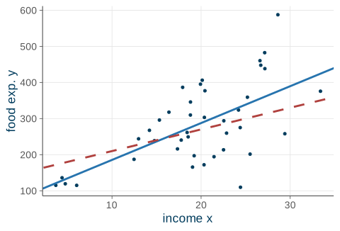
The first bad idea is freehand: just draw the line by eye. The trouble is that everyone draws a different line, and there is no rule by which to judge whose is best. The second bad idea is to use two endpoints: connect the lowest-income point to the highest-income point. That is at least a rule, but it throws away all the observations in between. What we want is a rule that uses every point and produces one answer. Figure 6.1 shows the food-expenditure cloud with two candidate lines passing through it; we need a principled way to say which is “best.”

Code

data(food)
ggplot(food, aes(income, food_exp)) +
  geom_point(color = ucla$darkblue, size = 1.1) +
  geom_abline(intercept = 83.42, slope = 10.21,
              color = ucla$blue, linewidth = 1) +
  geom_abline(intercept = 150, slope = 6,
              color = ucla$red, linetype = "dashed", linewidth = 1) +
  labs(x = "income x", y = "food exp. y")

Figure 6.1: Many lines pass through the data cloud. Which one is best?

Residuals: the vertical misses

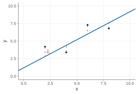
Fix any candidate line with intercept $b_1$ and slope $b_2$. Its fitted value at $x_i$ is \[ \hat y_i = b_1 + b_2 x_i , \] and the least squares residual is the vertical gap from the data point to the line: \[ \hat e_i = y_i - \hat y_i = y_i - b_1 - b_2 x_i . \] When $\hat e_i > 0$ the point lies above the line and we have under-predicted; when $\hat e_i < 0$ the point lies below it. A good line should make these misses small overall. Figure 6.2 shows the residuals as the dashed vertical segments connecting each point to the line.

Recall from the previous chapter that the residual $\hat e_i$ is the observable stand-in for the unobservable error $e_i$. We never see $e_i$, but once we have a fitted line we can compute every $\hat e_i$.

Code

pts <- data.frame(x = c(2, 4, 6, 8), y = c(4.2, 3.4, 7.3, 6.8))
pts$fit <- 1.2 + 0.8 * pts$x
ggplot(pts, aes(x, y)) +
  geom_abline(intercept = 1.2, slope = 0.8,
              color = ucla$blue, linewidth = 1) +
  geom_segment(aes(x = x, xend = x, y = y, yend = fit),
               color = ucla$red, linetype = "dashed") +
  geom_point(color = ucla$darkblue, size = 1.6) +
  annotate("text", x = 2.3, y = 3.5, label = "hat(e)[i]",
           parse = TRUE, color = ucla$red, size = 3.6) +
  scale_x_continuous(limits = c(0, 10)) +
  scale_y_continuous(limits = c(0, 10)) +
  labs(x = "x", y = "y")

Figure 6.2: Residuals are the dashed vertical segments from each point to the line.

The least squares criterion

Now we can state the rule.

The least squares principle

Choose the line that makes the sum of squared residuals as small as possible: \[ \min_{b_1, b_2}\; S(b_1, b_2) = \sum_{i=1}^{N} \hat e_i^{\,2} = \sum_{i=1}^{N}\bigl(y_i - b_1 - b_2 x_i\bigr)^2 . \]

Why squared distances? There are three good reasons. First, squaring makes every miss positive, so a large positive miss and a large negative miss cannot cancel each other out — which is exactly why we do not simply minimize $\sum \hat e_i$. Second, squaring penalizes big misses far more than small ones, so the line is pulled toward the bulk of the data. Third, it makes the minimization a clean calculus problem with a unique closed-form answer, which we derive in the next section.

What “least squares” buys us

Call the minimizing values $b_1, b_2$, and write the sum of squared residuals they achieve as \[ \mathrm{SSE} = \sum_{i=1}^{N} \hat e_i^{\,2}, \qquad \hat e_i = y_i - b_1 - b_2 x_i . \] For any other line $\hat y_i^{*} = b_1^{*} + b_2^{*} x_i$ with squared-residual total $\mathrm{SSE}^{*}$, we have \[ \boxed{\;\mathrm{SSE} \le \mathrm{SSE}^{*}\;} \qquad \text{(strict unless the lines coincide).} \] No matter how cleverly you draw an alternative, you cannot beat the least squares line on this criterion. The intercept and slope that achieve the minimum are the ordinary least squares (OLS) estimates.

“Ordinary” distinguishes OLS from variants — generalized, weighted, two-stage least squares — that you may meet later. There is nothing ordinary about how often it is used.

6.2 Deriving the OLS estimators

The objective $S(b_1, b_2) = \sum (y_i - b_1 - b_2 x_i)^2$ is a smooth, bowl-shaped (convex) function of two unknowns. Its minimum is the point where both partial derivatives vanish: \[ \begin{aligned} \frac{\partial S}{\partial b_1} &= -2 \sum \bigl(y_i - b_1 - b_2 x_i\bigr) = 0, \\[4pt] \frac{\partial S}{\partial b_2} &= -2 \sum x_i \bigl(y_i - b_1 - b_2 x_i\bigr) = 0 . \end{aligned} \] Dropping the common factor of $-2$ and rearranging gives the two normal equations: \[ \sum y_i = N b_1 + b_2 \sum x_i, \qquad \sum x_i y_i = b_1 \sum x_i + b_2 \sum x_i^2 . \] These are two linear equations in the two unknowns $(b_1, b_2)$, so we can solve them.

Notice that each first-order condition is a statement about residuals: $\sum \hat e_i = 0$ and $\sum x_i \hat e_i = 0$. The least squares residuals sum to zero and are uncorrelated with $x$ by construction — a fact we will lean on repeatedly.

Solving for the intercept

Take the first normal equation, $\sum y_i = N b_1 + b_2 \sum x_i$, and divide through by $N$: \[ \bar y = b_1 + b_2 \bar x \quad\Longrightarrow\quad \boxed{\,b_1 = \bar y - b_2 \bar x\,}. \]

The fitted line passes through the point of the means

Rearranged, the relationship reads $\bar y = b_1 + b_2 \bar x$: the OLS line always goes through $(\bar x, \bar y)$. The “point of the means” is a pivot — the line is anchored there and tilts to the best slope.

So once we know the slope $b_2$, the intercept is immediate. The real work is the slope.

Solving for the slope

Substitute $b_1 = \bar y - b_2 \bar x$ into the second normal equation and collect terms (the algebra is worked out in HGL Appendix 2A). The result, in deviation-from-means form, is \[ \boxed{\; b_2 = \frac{\sum_{i=1}^N (x_i - \bar x)(y_i - \bar y)} {\sum_{i=1}^N (x_i - \bar x)^2} \;} \] The numerator measures how $x$ and $y$ co-move about their means; the denominator measures how much $x$ varies about its mean. For this to be well-defined we need $\sum (x_i - \bar x)^2 \neq 0$ — which is precisely assumption SR5, that $x$ takes at least two distinct values. Without it the slope is $0/0$.

Sign of the slope

$b_2$ has the same sign as the sample covariance of $x$ and $y$: positive co-movement gives an upward-sloping fit, negative co-movement a downward-sloping one.

The slope is a ratio of sample moments

Divide the top and bottom of the slope formula by $N - 1$. The numerator becomes the sample covariance and the denominator the sample variance of $x$: \[ b_2 = \frac{\tfrac{1}{N-1} \sum (x_i - \bar x)(y_i - \bar y)} {\tfrac{1}{N-1} \sum (x_i - \bar x)^2} = \frac{\widehat{\Cov}(x, y)}{\widehat{\Var}(x)} . \]

An echo from the probability chapters

When we studied the bivariate Normal we found the population regression slope \[ \beta_2 = \frac{\Cov(X, Y)}{\Var(X)} . \] OLS is the sample analog: replace the population moments with their sample counterparts. The estimator mirrors the parameter, moment for moment — this is the analogy principle at work.

Estimator versus estimate, one more time

The formulas $b_2 = \dfrac{\sum (x_i - \bar x)(y_i - \bar y)}{\sum (x_i - \bar x)^2}$ and $b_1 = \bar y - b_2 \bar x$ are perfectly general — they work for whatever data turn up. That generality is exactly why the same symbols carry two meanings.

Two readings of $b_1$ and $b_2$

As formulas, they are estimators. Viewed as rules to be applied to a random sample, $b_1$ and $b_2$ are themselves random variables with a sampling distribution. That distribution is the subject of the next chapter.
As plugged-in numbers, they are estimates. Applied to one observed sample, they produce numbers ($b_2 = 10.21$, and so on). Just numbers — not random.

Same symbol, two meanings. Keeping them apart is the through-line of the whole course.

6.3 The food-expenditure example

To make all of this concrete we use the food data file from HGL: $N = 40$ three-person households. For each household we record $y_i$, weekly food expenditure in dollars, and $x_i$, weekly income measured in $100 units. A few rows and the column means look like this:

A few households from the `food` data, with the column means.
household	$y_i$	$x_i$
1	115.22	3.69
2	135.98	4.39
$\vdots$	$\vdots$	$\vdots$
40	375.73	33.40
mean	283.57	19.60

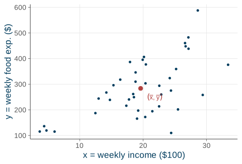
Figure 6.3 plots the full sample, with the point of the means $(\bar x, \bar y) = (19.60, 283.57)$ marked in red — the pivot the fitted line must pass through.

Code

xbar <- mean(food$income)
ybar <- mean(food$food_exp)
ggplot(food, aes(income, food_exp)) +
  geom_point(color = ucla$darkblue, size = 1.1) +
  annotate("point", x = xbar, y = ybar, color = ucla$red, size = 2.6) +
  annotate("text", x = xbar + 1, y = ybar - 35,
           label = "(bar(x) * ',' ~ bar(y))", parse = TRUE,
           color = ucla$red, size = 3.4, hjust = 0) +
  labs(x = "x = weekly income ($100)", y = "y = weekly food exp. ($)")

Figure 6.3: The food-expenditure data; the red dot is the point of the means.

Turning the crank

Plug the sample sums into the formulas (this reproduces HGL Example 2.4): \[ b_2 = \frac{\sum (x_i - \bar x)(y_i - \bar y)}{\sum (x_i - \bar x)^2} = \frac{18671.2684}{1828.7876} = 10.2096 , \] \[ b_1 = \bar y - b_2 \bar x = 283.5735 - (10.2096)(19.6048) = 83.4160 . \]

The fitted regression line

\[ \widehat{\text{FOOD\_EXP}}_i = 83.42 + 10.21\,\text{INCOME}_i \]

This is the line: of all possible lines it minimizes $\sum \hat e_i^2$, and it passes through $(\bar x, \bar y) = (19.60, 283.57)$.

Interpreting the estimates

The slope $b_2 = 10.21$ is the “how much” number. Because income is measured in $100 units, it says that a $100 rise in weekly income is associated with about $10.21 more weekly food spending, on average, holding everything else fixed. The intercept $b_1 = 83.42$ is, literally, predicted food spending at zero income.

Don't take the intercept literally

We have no data anywhere near $x = 0$ — the poorest household in the sample earns about $369 per week. Reading $b_1$ as “food spending for a household with no income at all” extrapolates far outside the data. Read it instead as the height that pins down the line.

Point prediction

For a household with $2{,}000 in weekly income ($x_0 = 20$, since income is in $100 units): \[ \hat y_0 = 83.42 + 10.21(20) = 287.61 . \] We predict $287.61 of weekly food spending. How sure are we about that number? That is a question for a prediction interval — see variance and prediction and prediction and fit.

Elasticity: a unit-free reading

A slope depends on the units of measurement. An elasticity — the percent change in $y$ per percent change in $x$ — does not. On a line the elasticity is \[ \hat\varepsilon = b_2 \cdot \frac{x}{\hat y}, \] which changes as we move along the line, so we report it at the representative point of the means: \[ \hat\varepsilon = 10.21 \times \frac{19.60}{283.57} = 0.71 . \]

Reading the elasticity

A 1% rise in income is associated with about a 0.71% rise in food spending. Because $0.71 < 1$, food is a necessity — demand grows less than proportionately with income — which is exactly what economic theory predicts.

6.4 OLS in R

You will almost never compute $b_1$ and $b_2$ by hand again. In R the workhorse is lm() (“linear model”). Read the formula food_exp ~ income as “regress food_exp on income.” R minimizes $\sum \hat e_i^2$ for you and returns the same $b_1 = 83.42$, $b_2 = 10.21$ we found by hand.

data(food)                            # course data package, loaded via POE5Rdata
fit <- lm(food_exp ~ income, data = food)
coef(fit)
#> (Intercept)      income 
#>    83.41600    10.20964

The fuller picture comes from summary(), which reports a whole table of quantities for each coefficient:

summary(fit)
#> 
#> Call:
#> lm(formula = food_exp ~ income, data = food)
#> 
#> Residuals:
#>      Min       1Q   Median       3Q      Max 
#> -223.025  -50.816   -6.324   67.879  212.044 
#> 
#> Coefficients:
#>             Estimate Std. Error t value Pr(>|t|)    
#> (Intercept)   83.416     43.410   1.922   0.0622 .  
#> income        10.210      2.093   4.877 1.95e-05 ***
#> ---
#> Signif. codes:  0 '***' 0.001 '**' 0.01 '*' 0.05 '.' 0.1 ' ' 1
#> 
#> Residual standard error: 89.52 on 38 degrees of freedom
#> Multiple R-squared:  0.385,  Adjusted R-squared:  0.3688 
#> F-statistic: 23.79 on 1 and 38 DF,  p-value: 1.946e-05

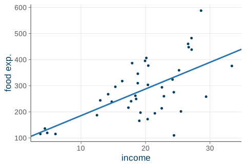
The Estimate column holds the $b$’s — our $83.42$ and $10.21$. The Std. Error column reports how much each estimate would wobble across repeated samples, which we study in the next chapter and variance and prediction. The remaining quantities — the $t$ statistics, $p$-values, and $R^2$ — belong to confidence intervals, hypothesis testing, and prediction and fit.

Finally, we can plot the data with the fitted line laid over it. Figure 6.4 shows the OLS line through the food-expenditure cloud.

Code

ggplot(food, aes(income, food_exp)) +
  geom_point(color = ucla$darkblue, size = 1.1) +
  geom_abline(intercept = coef(fit)[1], slope = coef(fit)[2],
              color = ucla$blue, linewidth = 1) +
  labs(x = "income", y = "food exp.")

Figure 6.4: The OLS line $\widehat{\text{food\_exp}} = 83.42 + 10.21\,\text{income}$ through the data.

6.5 Recap

The least squares principle chooses the line that minimizes the sum of squared residuals. We square the residuals so that positive and negative misses cannot cancel, and the resulting line beats every alternative on this criterion: $\mathrm{SSE} \le \mathrm{SSE}^{*}$.

Setting the two partial derivatives to zero gives the normal equations, which solve to the OLS estimators: \[ b_2 = \frac{\sum (x_i - \bar x)(y_i - \bar y)}{\sum (x_i - \bar x)^2} = \frac{\widehat{\Cov}(x, y)}{\widehat{\Var}(x)}, \qquad b_1 = \bar y - b_2 \bar x , \] and the fitted line always passes through the point of the means $(\bar x, \bar y)$.

For the food-expenditure data this yields \[ \widehat{\text{FOOD\_EXP}} = 83.42 + 10.21\,\text{INCOME}, \] so each extra $100 of weekly income is associated with about $10.21 more food spending; the elasticity at the means is $0.71$, marking food as a necessity. In R the whole calculation is one line: lm(food_exp ~ income).

Next time: we have a line, but $b_1$ and $b_2$ are random variables — so is the procedure unbiased, and how precise is it? In properties of OLS we show that OLS is unbiased and, under assumptions SR1–SR5, the best linear unbiased estimator (the Gauss–Markov theorem).

--- title: "OLS Estimation" --- {{< include _setup.qmd >}} > **Reading.** SW sec. 4.2, HGL sec. 2.3 In the [last chapter](05-simple-regression.qmd) we wrote down the simple linear regression model and its assumptions, but we never actually fit the line. The model is $$ y_i = \beta_1 + \beta_2 x_i + e_i, \qquad \E(y \given x) = \beta_1 + \beta_2 x , $$ where the parameters $\beta_1$ and $\beta_2$ are **fixed but unknown**. All we have is a sample of $N$ points $(x_i, y_i)$. This chapter turns that sample into numbers. We state the **least squares principle** --- the rule for choosing a line --- **derive** the estimators $b_2 = \widehat{\Cov}(x,y)/\widehat{\Var}(x)$ and $b_1 = \bar y - b_2 \bar x$, and **compute** them for the food-expenditure data, both by hand and in R. ::: {.keyidea title="The one-sentence preview"} OLS picks the line that makes the residuals as small as possible --- and the answer turns out to be just a ratio of sample moments you already met when we studied [covariance and correlation](03-expectation.qmd). ::: ## The least squares principle {#sec-least-squares} We want to locate the population mean line $\E(y \given x) = \beta_1 + \beta_2 x$ somewhere in the middle of the data cloud. Before stating the rule we actually use, it helps to see why two tempting shortcuts fail. The first bad idea is **freehand**: just draw the line by eye. The trouble is that everyone draws a different line, and there is no rule by which to judge whose is best. The second bad idea is to use **two endpoints**: connect the lowest-income point to the highest-income point. That is at least a rule, but it throws away all the observations in between. What we want is a rule that **uses every point** and produces **one** answer. @fig-which-line shows the food-expenditure cloud with two candidate lines passing through it; we need a principled way to say which is "best." ```{r} #| label: fig-which-line #| fig-cap: "Many lines pass through the data cloud. Which one is best?" #| fig-width: 5 #| fig-height: 3.4 data(food) ggplot(food, aes(income, food_exp)) + geom_point(color = ucla$darkblue, size = 1.1) + geom_abline(intercept = 83.42, slope = 10.21, color = ucla$blue, linewidth = 1) + geom_abline(intercept = 150, slope = 6, color = ucla$red, linetype = "dashed", linewidth = 1) + labs(x = "income x", y = "food exp. y") ``` ### Residuals: the vertical misses Fix *any* candidate line with intercept $b_1$ and slope $b_2$. Its **fitted value** at $x_i$ is $$ \hat y_i = b_1 + b_2 x_i , $$ and the **least squares residual** is the vertical gap from the data point to the line: $$ \hat e_i = y_i - \hat y_i = y_i - b_1 - b_2 x_i . $$ When $\hat e_i > 0$ the point lies **above** the line and we have under-predicted; when $\hat e_i < 0$ the point lies **below** it. A good line should make these misses small *overall*. @fig-residuals shows the residuals as the dashed vertical segments connecting each point to the line. ::: {.callout-note appearance="simple"} Recall from the [previous chapter](05-simple-regression.qmd) that the residual $\hat e_i$ is the observable **stand-in** for the unobservable error $e_i$. We never see $e_i$, but once we have a fitted line we can compute every $\hat e_i$. ::: ```{r} #| label: fig-residuals #| fig-cap: "Residuals are the dashed vertical segments from each point to the line." #| fig-width: 5 #| fig-height: 3.4 pts <- data.frame(x = c(2, 4, 6, 8), y = c(4.2, 3.4, 7.3, 6.8)) pts$fit <- 1.2 + 0.8 * pts$x ggplot(pts, aes(x, y)) + geom_abline(intercept = 1.2, slope = 0.8, color = ucla$blue, linewidth = 1) + geom_segment(aes(x = x, xend = x, y = y, yend = fit), color = ucla$red, linetype = "dashed") + geom_point(color = ucla$darkblue, size = 1.6) + annotate("text", x = 2.3, y = 3.5, label = "hat(e)[i]", parse = TRUE, color = ucla$red, size = 3.6) + scale_x_continuous(limits = c(0, 10)) + scale_y_continuous(limits = c(0, 10)) + labs(x = "x", y = "y") ``` ### The least squares criterion Now we can state the rule. ::: {.keyidea title="The least squares principle"} Choose the line that makes the **sum of squared residuals** as small as possible: $$ \min_{b_1, b_2}\; S(b_1, b_2) = \sum_{i=1}^{N} \hat e_i^{\,2} = \sum_{i=1}^{N}\bigl(y_i - b_1 - b_2 x_i\bigr)^2 . $$ ::: Why *squared* distances? There are three good reasons. First, squaring makes every miss positive, so a large positive miss and a large negative miss cannot **cancel** each other out --- which is exactly why we do not simply minimize $\sum \hat e_i$. Second, squaring penalizes **big** misses far more than small ones, so the line is pulled toward the bulk of the data. Third, it makes the minimization a clean calculus problem with a **unique** closed-form answer, which we derive in the [next section](#sec-deriving). ### What "least squares" buys us Call the minimizing values $b_1, b_2$, and write the sum of squared residuals they achieve as $$ \mathrm{SSE} = \sum_{i=1}^{N} \hat e_i^{\,2}, \qquad \hat e_i = y_i - b_1 - b_2 x_i . $$ For *any* other line $\hat y_i^{*} = b_1^{*} + b_2^{*} x_i$ with squared-residual total $\mathrm{SSE}^{*}$, we have $$ \boxed{\;\mathrm{SSE} \le \mathrm{SSE}^{*}\;} \qquad \text{(strict unless the lines coincide).} $$ No matter how cleverly you draw an alternative, you cannot beat the least squares line on this criterion. The intercept and slope that achieve the minimum are the **ordinary least squares** (OLS) estimates. ::: {.callout-note appearance="simple"} "Ordinary" distinguishes OLS from variants --- generalized, weighted, two-stage least squares --- that you may meet later. There is nothing ordinary about how often it is used. ::: ## Deriving the OLS estimators {#sec-deriving} The objective $S(b_1, b_2) = \sum (y_i - b_1 - b_2 x_i)^2$ is a smooth, bowl-shaped (convex) function of two unknowns. Its minimum is the point where both partial derivatives vanish: $$ \begin{aligned} \frac{\partial S}{\partial b_1} &= -2 \sum \bigl(y_i - b_1 - b_2 x_i\bigr) = 0, \\[4pt] \frac{\partial S}{\partial b_2} &= -2 \sum x_i \bigl(y_i - b_1 - b_2 x_i\bigr) = 0 . \end{aligned} $$ Dropping the common factor of $-2$ and rearranging gives the two **normal equations**: $$ \sum y_i = N b_1 + b_2 \sum x_i, \qquad \sum x_i y_i = b_1 \sum x_i + b_2 \sum x_i^2 . $$ These are two linear equations in the two unknowns $(b_1, b_2)$, so we can solve them. ::: {.callout-note appearance="simple"} Notice that each first-order condition is a statement about residuals: $\sum \hat e_i = 0$ and $\sum x_i \hat e_i = 0$. The least squares residuals sum to zero and are uncorrelated with $x$ **by construction** --- a fact we will lean on repeatedly. ::: ### Solving for the intercept Take the first normal equation, $\sum y_i = N b_1 + b_2 \sum x_i$, and divide through by $N$: $$ \bar y = b_1 + b_2 \bar x \quad\Longrightarrow\quad \boxed{\,b_1 = \bar y - b_2 \bar x\,}. $$ ::: {.property title="The fitted line passes through the point of the means"} Rearranged, the relationship reads $\bar y = b_1 + b_2 \bar x$: the OLS line always goes through $(\bar x, \bar y)$. The "point of the means" is a pivot --- the line is anchored there and tilts to the best slope. ::: So once we know the slope $b_2$, the intercept is immediate. The real work is the slope. ### Solving for the slope Substitute $b_1 = \bar y - b_2 \bar x$ into the second normal equation and collect terms (the algebra is worked out in HGL Appendix 2A). The result, in **deviation-from-means** form, is $$ \boxed{\; b_2 = \frac{\sum_{i=1}^N (x_i - \bar x)(y_i - \bar y)} {\sum_{i=1}^N (x_i - \bar x)^2} \;} $$ The numerator measures how $x$ and $y$ **co-move** about their means; the denominator measures how much $x$ **varies** about its mean. For this to be well-defined we need $\sum (x_i - \bar x)^2 \neq 0$ --- which is precisely assumption **SR5**, that $x$ takes at least two distinct values. Without it the slope is $0/0$. ::: {.property title="Sign of the slope"} $b_2$ has the same sign as the sample covariance of $x$ and $y$: positive co-movement gives an upward-sloping fit, negative co-movement a downward-sloping one. ::: ### The slope *is* a ratio of sample moments Divide the top and bottom of the slope formula by $N - 1$. The numerator becomes the **sample covariance** and the denominator the **sample variance** of $x$: $$ b_2 = \frac{\tfrac{1}{N-1} \sum (x_i - \bar x)(y_i - \bar y)} {\tfrac{1}{N-1} \sum (x_i - \bar x)^2} = \frac{\widehat{\Cov}(x, y)}{\widehat{\Var}(x)} . $$ ::: {.keyidea title="An echo from the probability chapters"} When we studied the bivariate Normal we found the population regression slope $$ \beta_2 = \frac{\Cov(X, Y)}{\Var(X)} . $$ OLS is the **sample analog**: replace the population moments with their sample counterparts. The estimator mirrors the parameter, moment for moment --- this is the **analogy principle** at work. ::: ### Estimator versus estimate, one more time The formulas $b_2 = \dfrac{\sum (x_i - \bar x)(y_i - \bar y)}{\sum (x_i - \bar x)^2}$ and $b_1 = \bar y - b_2 \bar x$ are **perfectly general** --- they work for whatever data turn up. That generality is exactly why the same symbols carry two meanings. ::: {.definition title="Two readings of $b_1$ and $b_2$"} - **As formulas, they are estimators.** Viewed as rules to be applied to a *random* sample, $b_1$ and $b_2$ are themselves **random variables** with a sampling distribution. That distribution is the subject of [the next chapter](07-ols-properties.qmd). - **As plugged-in numbers, they are estimates.** Applied to *one* observed sample, they produce numbers ($b_2 = 10.21$, and so on). Just numbers --- not random. ::: Same symbol, two meanings. Keeping them apart is the through-line of the whole course. ## The food-expenditure example {#sec-food-example} To make all of this concrete we use the `food` data file from HGL: $N = 40$ three-person households. For each household we record $y_i$, weekly food expenditure in dollars, and $x_i$, weekly income measured in \$100 units. A few rows and the column means look like this: | household | $y_i$ | $x_i$ | |----------:|------:|------:| | 1 | 115.22 | 3.69 | | 2 | 135.98 | 4.39 | | $\vdots$ | $\vdots$ | $\vdots$ | | 40 | 375.73 | 33.40 | | **mean** | **283.57** | **19.60** | : A few households from the `food` data, with the column means. {.striped} @fig-food-scatter plots the full sample, with the point of the means $(\bar x, \bar y) = (19.60, 283.57)$ marked in red --- the pivot the fitted line must pass through. ```{r} #| label: fig-food-scatter #| fig-cap: "The food-expenditure data; the red dot is the point of the means." #| fig-width: 5 #| fig-height: 3.4 xbar <- mean(food$income) ybar <- mean(food$food_exp) ggplot(food, aes(income, food_exp)) + geom_point(color = ucla$darkblue, size = 1.1) + annotate("point", x = xbar, y = ybar, color = ucla$red, size = 2.6) + annotate("text", x = xbar + 1, y = ybar - 35, label = "(bar(x) * ',' ~ bar(y))", parse = TRUE, color = ucla$red, size = 3.4, hjust = 0) + labs(x = "x = weekly income ($100)", y = "y = weekly food exp. ($)") ``` ### Turning the crank Plug the sample sums into the formulas (this reproduces HGL Example 2.4): $$ b_2 = \frac{\sum (x_i - \bar x)(y_i - \bar y)}{\sum (x_i - \bar x)^2} = \frac{18671.2684}{1828.7876} = 10.2096 , $$ $$ b_1 = \bar y - b_2 \bar x = 283.5735 - (10.2096)(19.6048) = 83.4160 . $$ ::: {.property title="The fitted regression line"} $$ \widehat{\text{FOOD\_EXP}}_i = 83.42 + 10.21\,\text{INCOME}_i $$ ::: This is *the* line: of all possible lines it minimizes $\sum \hat e_i^2$, and it passes through $(\bar x, \bar y) = (19.60, 283.57)$. ### Interpreting the estimates The **slope** $b_2 = 10.21$ is the "how much" number. Because income is measured in \$100 units, it says that a **\$100 rise in weekly income** is associated with about **\$10.21 more** weekly food spending, on average, holding everything else fixed. The **intercept** $b_1 = 83.42$ is, literally, predicted food spending at **zero income**. ::: {.warningbox title="Don't take the intercept literally"} We have **no data** anywhere near $x = 0$ --- the poorest household in the sample earns about \$369 per week. Reading $b_1$ as "food spending for a household with no income at all" extrapolates far outside the data. Read it instead as the height that pins down the line. ::: ::: {.example title="Point prediction"} For a household with \$2{,}000 in weekly income ($x_0 = 20$, since income is in \$100 units): $$ \hat y_0 = 83.42 + 10.21(20) = 287.61 . $$ We predict \$287.61 of weekly food spending. *How sure* are we about that number? That is a question for a prediction interval --- see [variance and prediction](08-variance-prediction.qmd) and [prediction and fit](11-prediction-fit.qmd). ::: ### Elasticity: a unit-free reading A slope depends on the units of measurement. An **elasticity** --- the percent change in $y$ per percent change in $x$ --- does not. On a line the elasticity is $$ \hat\varepsilon = b_2 \cdot \frac{x}{\hat y}, $$ which changes as we move along the line, so we report it at the representative point of the means: $$ \hat\varepsilon = 10.21 \times \frac{19.60}{283.57} = 0.71 . $$ ::: {.keyidea title="Reading the elasticity"} A 1\% rise in income is associated with about a **0.71\%** rise in food spending. Because $0.71 < 1$, food is a **necessity** --- demand grows less than proportionately with income --- which is exactly what economic theory predicts. ::: ## OLS in R {#sec-ols-in-r} You will almost never compute $b_1$ and $b_2$ by hand again. In R the workhorse is `lm()` ("linear model"). Read the formula `food_exp ~ income` as "regress `food_exp` **on** `income`." R minimizes $\sum \hat e_i^2$ for you and returns the same $b_1 = 83.42$, $b_2 = 10.21$ we found by hand. ```{r} #| code-fold: false data(food) # course data package, loaded via POE5Rdata fit <- lm(food_exp ~ income, data = food) coef(fit) ``` The fuller picture comes from `summary()`, which reports a whole table of quantities for each coefficient: ```{r} #| code-fold: false summary(fit) ``` The **`Estimate`** column holds the $b$'s --- our $83.42$ and $10.21$. The **`Std. Error`** column reports how much each estimate would wobble across repeated samples, which we study in [the next chapter](07-ols-properties.qmd) and [variance and prediction](08-variance-prediction.qmd). The remaining quantities --- the $t$ statistics, $p$-values, and $R^2$ --- belong to [confidence intervals](09-confidence-intervals.qmd), [hypothesis testing](10-hypothesis-testing.qmd), and [prediction and fit](11-prediction-fit.qmd). Finally, we can plot the data with the fitted line laid over it. @fig-food-fit shows the OLS line through the food-expenditure cloud. ```{r} #| label: fig-food-fit #| fig-cap: "The OLS line $\\widehat{\\text{food\\_exp}} = 83.42 + 10.21\\,\\text{income}$ through the data." #| fig-width: 5 #| fig-height: 3.4 ggplot(food, aes(income, food_exp)) + geom_point(color = ucla$darkblue, size = 1.1) + geom_abline(intercept = coef(fit)[1], slope = coef(fit)[2], color = ucla$blue, linewidth = 1) + labs(x = "income", y = "food exp.") ``` ## Recap {#sec-recap} The **least squares principle** chooses the line that minimizes the sum of squared residuals. We square the residuals so that positive and negative misses cannot cancel, and the resulting line beats every alternative on this criterion: $\mathrm{SSE} \le \mathrm{SSE}^{*}$. Setting the two partial derivatives to zero gives the normal equations, which solve to the **OLS estimators**: $$ b_2 = \frac{\sum (x_i - \bar x)(y_i - \bar y)}{\sum (x_i - \bar x)^2} = \frac{\widehat{\Cov}(x, y)}{\widehat{\Var}(x)}, \qquad b_1 = \bar y - b_2 \bar x , $$ and the fitted line always passes through the point of the means $(\bar x, \bar y)$. For the food-expenditure data this yields $$ \widehat{\text{FOOD\_EXP}} = 83.42 + 10.21\,\text{INCOME}, $$ so each extra \$100 of weekly income is associated with about \$10.21 more food spending; the elasticity at the means is $0.71$, marking food as a necessity. In R the whole calculation is one line: `lm(food_exp ~ income)`. **Next time:** we have *a* line, but $b_1$ and $b_2$ are random variables --- so is the procedure **unbiased**, and how **precise** is it? In [properties of OLS](07-ols-properties.qmd) we show that OLS is unbiased and, under assumptions SR1--SR5, the **best linear unbiased estimator** (the Gauss--Markov theorem).